Lecture 2: Surface Flux & Colors of Stars
How hot, how big? From luminosity and color to temperature and radius
Learning Objectives
After completing this reading, you should be able to:
- Distinguish between received flux (what an observer measures) and surface flux (a stellar property)
- Explain why surface brightness is independent of distance using inverse-square scaling
- Apply the Stefan-Boltzmann law: \(L = 4\pi R^2 \sigma T^4\) to connect luminosity, temperature, and radius
- Interpret the meaning and units of Stefan-Boltzmann constant \(\sigma = 5.67 \times 10^{-5}\) erg cm\(^{-2}\) s\(^{-1}\) K\(^{-4}\)
- Use Wien’s displacement law to infer stellar surface temperature from observed color
- Calculate stellar radius given measurements of luminosity and temperature
- Connect color sequence to temperature sequence and preview the HR diagram’s organization
Concept Throughline
Color is temperature. Luminosity, temperature, and radius form a closed relationship: know any two, infer the third.
By measuring a star’s color (from Wien’s law) and its luminosity (from flux plus distance), we can determine its physical size — the radius — without ever visiting the star. This is the power of blackbody physics applied to astronomy.
When we say “color is temperature,” we do not mean only the color your eyes perceive. We mean electromagnetic color — the peak wavelength of a star’s Planck curve across the entire electromagnetic spectrum, from radio waves through gamma rays. Rigel’s “color” peaks in the ultraviolet at ~240 nm; Betelgeuse’s peaks in the near-infrared at ~830 nm. Neither peak is visible to the human eye, yet both encode the star’s temperature through Wien’s law.
In practice, two additional complications matter: (1) interstellar dust scatters and absorbs blue light preferentially, making stars appear redder and cooler than they truly are (you’ll quantify this effect in Practice Problem 12), and (2) astronomers rarely measure the exact peak wavelength — instead they compare flux through standardized filters and infer an effective temperature from that ratio.
Bottom line: “Color” in this course means “where the Planck curve peaks” — a quantity defined across all wavelengths, not just the narrow visible band. The temperature we infer is always an effective temperature, and it requires corrections for dust before it’s reliable.
In HW3 and exams, we will treat color operationally as peak wavelength (or a close proxy) and use Wien’s law to infer \(T_{\text{eff}}\).
Track A (Core, ~25 min): Read Parts 1–6 in order — the main text, all four worked examples, Quick Checks, and the Common Student Confusions box. Skip any box marked Enrichment (these are collapsible and clearly labeled). This gives you every equation, technique, and concept you need for homework and exams.
Track B (Full, ~35 min): Read everything, including Enrichment boxes (historical context, the Wien caveat, OBAFGKM spectral types) and Parts 7–8 (HR diagram preview and assumptions/limitations). Part 8 won’t appear on exams, but it builds important context for later modules.
Both tracks cover all learning objectives. Track B adds depth that will pay off as we build the full HR diagram.
You already have the tools. In Lecture 4 (Module 1), you learned that color encodes temperature (Wien’s law) and that blackbodies follow \(B_\lambda(T)\) curves. In Lecture 1, you learned to measure luminosity from received flux and distance. Today we combine these into a complete inference: if you know a star’s color and its brightness from Earth, you can infer its size. This is how we learned that Betelgeuse is nearly 900 times the Sun’s radius.
What you’ll gain: By the end of this reading, you’ll be able to look at any star’s color and brightness and determine its temperature, luminosity, and physical size — without ever leaving Earth. That’s three fundamental properties from two measurements and one equation.
Part 1: Opening Hook — Two Stars with the Same Luminosity
The Puzzle
Step outside on a winter evening and look toward Orion. The constellation’s two brightest stars — blue-white Rigel at the foot and red Betelgeuse at the shoulder — appear similarly bright to your eye. It turns out their total luminosities are also comparable: each radiates roughly 100,000 times the Sun’s total power. Yet one is a compact blue supergiant and the other is an enormous red supergiant whose surface would extend past Mars’s orbit and nearly reach Jupiter’s. How can two stars with the same luminosity be so different in size?
Your intuition from everyday experience might say: “They’re equally bright, so they must be similar in size.” But that intuition is wrong for stars.
The catch: A hot (blue) object radiates energy much more efficiently per square centimeter than a cool (red) object. So to produce the same total luminosity, a hot star can be smaller than a cool star.
- A hot star: radiates a lot per unit area, so it doesn’t need to be as large
- A cool star: radiates little per unit area, so it must be huge to produce the same total
This lecture quantifies that intuition using the Stefan-Boltzmann law, and it’s the second major step in stellar inference. Combined with your knowledge of luminosity (Lecture 1) and color (Lecture 4 (Module 1)), you can now infer stellar radii.
- Observable: received flux (brightness from Earth) + distance → luminosity (Lecture 1)
- Observable: color (peak wavelength from spectrum) → temperature via Wien’s law (Lecture 4, Module 1)
- Model: Stefan-Boltzmann law connects \(L\), \(T\), and \(R\)
- Inference: given \(L\) and \(T\), solve for \(R\)
Part 2: Surface Flux vs. Received Flux
Received Flux: Distance-Dependent
In Lecture 1, you learned that the flux received at Earth is
\[ F = \frac{L}{4\pi d^2} \tag{1}\]
What it predicts
Given \(L\) and \(d\), it predicts the observed flux \(F\) at the detector.
What it depends on
Scales as \(F \propto L\) and \(F \propto d^{-2}\).
What it’s saying
Apparent brightness mixes intrinsic power and distance; to infer \(L\) from \(F\), you must also know \(d\).
Assumptions
- Approximately isotropic emission (radiates equally in all directions)
- Negligible absorption/scattering between source and observer
See: the equation
where \(L\) is the star’s luminosity and \(d\) is the distance.

Light intensity decreases with the square of distance (Credit: Course illustration (A. Rosen))
Key point: This flux depends on the observer’s distance. The farther you are, the dimmer it appears — even though the star’s intrinsic power hasn’t changed. As shown in the figure above, the same luminosity \(L\) is spread over a sphere of area \(4\pi d^2\) that grows with distance.
Surface Flux: Star-Dependent
Now consider a different question: if you could stand on the star’s surface, how much power per unit area would you receive?
That quantity is called the emitted (bolometric) surface flux:
\[F_* = \frac{L}{4\pi R^2}\]
where \(R\) is the star’s radius.
Key insight: Surface flux depends only on the star’s intrinsic properties (its total output \(L\) and its size \(R\)), not on where the observer is. An observer on the star’s equator always measures the same \(F_*\), regardless of whether someone else is observing from Earth.
| Quantity | Equation | What it measures | Depends on |
|---|---|---|---|
| Received flux (\(F\)) | \(F = L/(4\pi d^2)\) | Brightness we measure | Star’s distance; our location |
| Surface flux (\(F_*\)) | \(F_* = L/(4\pi R^2)\) | Radiation intensity at star’s surface | Star’s luminosity and radius only |
| Symbol | Name | Units (CGS) | Meaning |
|---|---|---|---|
| \(L\) | Luminosity | erg/s | Total power output of a star |
| \(F\) | Received flux | erg s\(^{-1}\) cm\(^{-2}\) | Power per unit area at distance \(d\) |
| \(F_*\) | Surface flux | erg s\(^{-1}\) cm\(^{-2}\) | Power per unit area at star’s surface |
| \(R\) | Stellar radius | cm (or \(R_\odot\)) | Physical size of the star |
| \(d\) | Distance | cm (or pc) | Observer-to-star distance |
| \(T\) | Effective temperature | K | Blackbody temperature matching total flux |
| \(\sigma\) | Stefan-Boltzmann constant | erg cm\(^{-2}\) s\(^{-1}\) K\(^{-4}\) | \(5.67 \times 10^{-5}\) |
| \(b\) | Wien’s constant | cm·K (or nm·K) | \(0.2898\) cm·K \(= 2.898 \times 10^6\) nm·K |
| \(\lambda_{\text{peak}}\) | Peak wavelength | nm or cm | Where the Planck curve peaks |
| \(B_\lambda(T)\) | Planck function | erg s\(^{-1}\) cm\(^{-2}\) sr\(^{-1}\) cm\(^{-1}\) | Spectral radiance (from Lecture 4, Module 1) |
| \(\Omega\) | Solid angle | sr (steradians) | Angular area subtended on the sky |
Subscript \(\odot\) denotes solar values: \(L_\odot\), \(R_\odot\), \(T_\odot\).
A useful relationship links received flux to surface flux. Dividing \(F = L/(4\pi d^2)\) by \(F_* = L/(4\pi R^2)\), the luminosity \(L\) and the factor \(4\pi\) cancel:
\[\frac{F}{F_*} = \frac{R^2}{d^2}\]
This single ratio encapsulates the geometry: the fraction of the surface flux that reaches you equals the square of the ratio of the star’s radius to your distance. Since \(R \ll d\) for every star, only a tiny fraction of the surface flux arrives at Earth.
- If a star’s distance doubles, received flux ___?
- If a star’s radius doubles (with \(L\) fixed), surface flux ___?
- Two stars have the same received flux at Earth. Does that mean they have the same surface flux?
- Quarters (divides by 4) — received flux scales as \(d^{-2}\)
- Quarters (divides by 4) — surface flux scales as \(R^{-2}\)
- No. Received flux depends on both luminosity and distance. Two stars with the same received flux could have different distances and luminosities, leading to different surface fluxes.
Surface Brightness is Independent of Distance (Optional Extension)
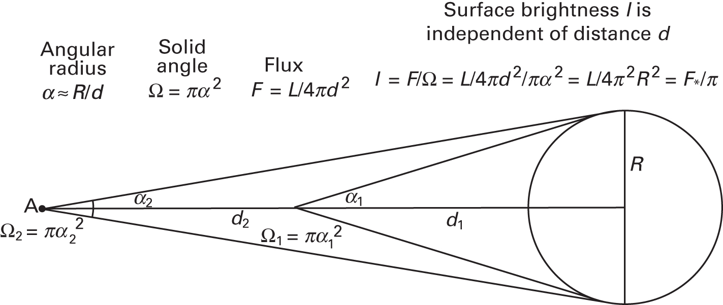
What to notice: Surface brightness is distance-independent because both received flux and apparent solid angle scale as \(1/d^2\), so their ratio stays constant. (Credit: Fundamentals of Astrophysics (Owocki))
Optional (Track B): You can skip this derivation for HW3 and exams. It becomes very useful later for galaxies, nebulae, and any resolved extended source.
Imagine looking at a star’s disk through a small telescope.
- Flux received: \(F \propto d^{-2}\) (inverse-square law)
- Solid angle subtended: \(\Omega \propto R^2 d^{-2}\) (the star looks smaller at distance; angular size is \(\theta \sim R/d\), and solid angle is \(\theta^2\))
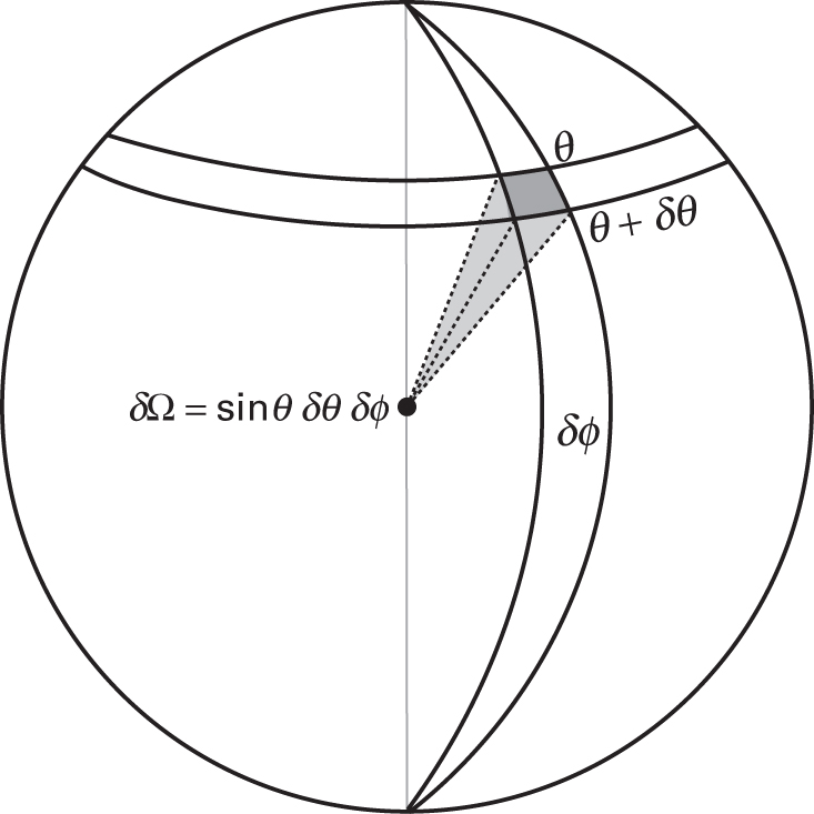
What to notice: A small patch on the sky has solid angle \(\delta\Omega=\sin\theta\,\delta\theta\,\delta\phi\), the 2D angular area element used in flux and intensity integrals. (Credit: Fundamentals of Astrophysics (Owocki))
- Surface brightness: \(\text{SB} = F/\Omega \propto (d^{-2})/(R^2 d^{-2}) = \text{constant}\)
The inverse-square decline in flux is exactly canceled by the inverse-square decline in solid angle, so the surface brightness (flux per unit solid angle) is independent of distance.
Important: This applies to resolved sources — objects whose angular extent you can measure (e.g., planet disks, galaxies, nebulae). Most stars are unresolved point sources in typical telescopes, but the principle is still essential for understanding extended objects.
For a uniform, isotropically emitting surface (Lambertian), the bolometric intensity is \(I = F_*/\pi\), so \(F/\Omega\) is distance-independent for resolved sources. You can’t determine a star’s distance just by measuring how bright it looks on the sky without additional information. A dim, distant star can appear to have the same surface brightness as a bright, nearby one.
This is why parallax (Lecture 1) and standard candles matter for distance — brightness alone isn’t enough.
A note on notation: We use \(\text{SB}\) for surface brightness (flux per solid angle) to avoid confusion with \(B_\lambda(T)\), which denotes the Planck function (spectral radiance) introduced in Lecture 4 (Module 1). These are related but distinct quantities.
Part 2 takeaway: Received flux tells you how bright a star appears from where you stand; surface flux tells you how much energy the star actually radiates per square centimeter of its surface. The first depends on distance; the second does not.
Before moving on, watch out for these pitfalls:
- Flux vs. luminosity: Flux (\(F\)) is power per unit area received at a specific distance; luminosity (\(L\)) is total power output. Same received flux does not imply same luminosity unless both stars are at the same distance.
- “Brightness” is ambiguous: In everyday language, “bright” could mean high luminosity, high received flux, or high surface brightness. In this course, always specify which quantity you mean.
- (Track B) Flux vs. intensity: Flux (\(F\)) is the total power per unit area arriving from all directions; intensity (\(I\)) is power per unit area per unit solid angle. They are related (\(F = \pi I\) for isotropic emission from a flat surface) but not interchangeable. You won’t need this distinction for exams, but it matters in the surface brightness derivation above.
Your lab partner claims: “If we moved Betelgeuse to the same distance as Sirius, they’d have the same received flux, so they must have the same surface flux too.” Construct a counterargument. Which quantities in the claim are distance-dependent, and which are intrinsic to the star? Use the relationship \(F/F_* = R^2/d^2\) to explain why equal received flux does not imply equal surface flux.
Check Yourself
Before reading further, make sure you can answer:
- What is the difference between “luminosity” and “received flux”? (From Lecture 1: luminosity is total power output; flux is power per unit area received at Earth.)
- What is the definition of “surface flux,” and why does it not depend on distance?
- If a star’s radius doubled but its luminosity stayed the same, would the surface flux increase, decrease, or stay the same?
Part 3: The Stefan-Boltzmann Law — From Temperature to Luminosity
The Law
Every blackbody is fundamentally described by its temperature \(T\). The Stefan-Boltzmann law quantifies how much power a blackbody of a given temperature radiates per unit area:
\[F_* = \sigma T^4\]
where \(\sigma = 5.67 \times 10^{-5}\) erg cm\(^{-2}\) s\(^{-1}\) K\(^{-4}\) is the Stefan-Boltzmann constant.
Units sanity check: \(\sigma\) is “power per area per \(T^4\)” so \(\sigma T^4\) has units of flux (erg cm\(^{-2}\) s\(^{-1}\)).
This tells us the surface flux — the power radiated per unit area — in terms of temperature alone.
To get the total luminosity, recall the definition from Part 2: \(L = F_* \times (\text{surface area})\). For a sphere, the surface area is \(4\pi R^2\). Substituting \(F_* = \sigma T^4\):
\[L = F_* \times 4\pi R^2 = \sigma T^4 \times 4\pi R^2 = 4\pi R^2 \sigma T^4\]
\[ L = 4\pi R^2 \sigma T^4 \tag{2}\]
What it predicts
Given \(R\) and \(T\), it predicts the luminosity \(L\).
What it depends on
Scales as \(L \propto R^2 T^4\).
What it’s saying
Luminosity depends on surface area (\(R^2\)) and temperature (\(T^4\)). Double the temperature, get 16× the luminosity.
Assumptions
- Blackbody radiation
- Spherical, uniformly radiating surface
- Effective surface temperature
See: the equation
Unpacking the Stefan-Boltzmann Law
Let’s interpret this equation piece by piece:
The story — Temperature dominates; size amplifies: - A hot object radiates much more power per unit area than a cool object (temperature appears as \(T^4\)) - The total power radiated is proportional to surface area (\(4\pi R^2\)) - Together: the hotter something is, and the larger it is, the more power it radiates
What it depends on: - \(T\) (surface temperature) — increases as \(T^4\), so very steep dependence - \(R\) (radius) — increases as \(R^2\), quadratic - Nothing else (assuming uniform temperature and spherical symmetry)
Physical meaning of each piece: - \(4\pi R^2\) = surface area of a sphere (geometry) - \(\sigma T^4\) = power radiated per unit area at temperature \(T\) (blackbody physics) - The product = total power output
What to notice: Hotter stars peak at shorter wavelengths (bluer) AND emit more total light. A blue 8000 K star peaks near \(\lambda_{\mathrm{peak}}\approx 360\ \mathrm{nm}\); a red 3000 K star peaks near \(970\ \mathrm{nm}\). Wien’s law: \(\lambda_{\mathrm{peak}} = b/T\) with \(b = 0.2898\) cm·K. (Credit: JWST/STScI)
\[[L] = [R^2] \times [\sigma T^4] = \text{cm}^2 \times \frac{\text{erg}}{\text{cm}^2 \cdot \text{s} \cdot \text{K}^4} \times \text{K}^4 = \frac{\text{erg}}{\text{s}} = \text{erg/s}\ \checkmark\]
Notice how the cm\(^2\) cancels, the K\(^4\) cancels, and we’re left with erg/s — units of power, as required.
Stefan-Boltzmann constant in cgs: \[\sigma = 5.67 \times 10^{-5}\ \text{erg}\ \text{cm}^{-2}\ \text{s}^{-1}\ \text{K}^{-4}\]
Read the negative exponents carefully: cm\(^{-2}\) means “per square centimeter,” s\(^{-1}\) means “per second,” K\(^{-4}\) means “per kelvin to the fourth power.” Memorize this number or know where to find it. It’s as fundamental as \(G\) or \(c\).
Three Variables, One Equation: The Key Insight
The Stefan-Boltzmann law connects three quantities: \(L\), \(T\), and \(R\). If you know any two, you can solve for the third.
\[\text{Given } L \text{ and } T: \quad R = \left(\frac{L}{4\pi\sigma T^4}\right)^{1/2}\]
\[\text{Given } R \text{ and } T: \quad L = 4\pi R^2 \sigma T^4\]
\[\text{Given } L \text{ and } R: \quad T = \left(\frac{L}{4\pi\sigma R^2}\right)^{1/4}\]
Notation convention: Throughout this reading, we write fractional powers rather than root symbols: \(x^{1/2}\) instead of \(\sqrt{x}\), \(x^{1/4}\) instead of \(\sqrt[4]{x}\). This convention generalizes cleanly — you’ll encounter \(1/3\) and \(1/4\) powers in later modules — and it makes algebraic manipulation easier (e.g., \((x^{1/2})^2 = x^1 = x\)). Both notations mean the same thing; the exponent form is what you should use in your own work.
This is powerful because:
- Luminosity can be inferred from received flux + distance (Lecture 1)
- Temperature can be inferred from color via Wien’s law (Lecture 4 (Module 1))
- Therefore, radius can be inferred from the Stefan-Boltzmann law
By Lecture 2, you have three measurable quantities: 1. Brightness from Earth → distance (parallax, Lecture 1) + brightness → luminosity 2. Color of the star → temperature (Wien’s law, Lecture 4 (Module 1)) 3. Stefan-Boltzmann law → radius
Three observables, three inferences. This is how we built a census of stellar radii without ever landing on a star.
From \(L = 4\pi R^2 \sigma T^4\), we can extract powerful proportionalities:
- For fixed luminosity (comparing two stars with the same \(L\)): \(R \propto T^{-2}\). A star twice as hot needs only \(1/4\) the radius to produce the same luminosity.
- For fixed radius (same-size stars at different temperatures): \(L \propto T^{4}\). A star twice as hot is \(2^4 = 16\times\) more luminous.
- For fixed temperature (same-temperature stars of different sizes): \(L \propto R^{2}\). A star twice as large is \(4\times\) more luminous.
Error sensitivity: Since \(R \propto L^{1/2}\,T^{-2}\) (at fixed \(L\), isolating \(R\)), temperature errors propagate steeply:
\[\frac{\Delta R}{R} \approx \frac{1}{2}\frac{\Delta L}{L} + 2\frac{\Delta T}{T}\]
A 10% error in temperature produces a ~20% error in the inferred radius. Temperature matters a lot!
Part 3 takeaway: The Stefan-Boltzmann law \(L = 4\pi R^2 \sigma T^4\) is the bridge between observable quantities and physical size. Temperature enters as \(T^4\) — a steep dependence that makes even small temperature differences produce large effects.
Part 4: Dimensionless Form — Scaling Relations with the Sun
Working with the Stefan-Boltzmann law in absolute CGS units means juggling numbers like \(\sigma = 5.67 \times 10^{-5}\) and \(R_\odot = 6.96 \times 10^{10}\) cm — easy places for arithmetic errors to creep in. There’s a much cleaner approach: express everything relative to the Sun. Since the Sun is a well-characterized star whose luminosity, radius, and temperature are precisely known, it serves as a natural benchmark. Dividing the Stefan-Boltzmann law for any star by the same law applied to the Sun cancels the constants and yields a dimensionless scaling relation.
For easy comparison, we express luminosity, radius, and temperature in solar units:
\[\frac{L}{L_\odot} = \left(\frac{R}{R_\odot}\right)^2 \left(\frac{T}{T_\odot}\right)^4\]
To derive this, write the Stefan-Boltzmann law for any star and for the Sun, then divide:
\[\frac{L}{L_\odot} = \frac{4\pi R^2 \sigma T^4}{4\pi R_\odot^2 \sigma T_\odot^4}\]
Notice that \(4\pi\) and \(\sigma\) appear in both the numerator and denominator, so they cancel — leaving only ratios of stellar properties:
\[\frac{L}{L_\odot} = \frac{R^2}{R_\odot^2} \cdot \frac{T^4}{T_\odot^4} = \left(\frac{R}{R_\odot}\right)^2 \left(\frac{T}{T_\odot}\right)^4\]
This is the payoff: constants disappear, and you work entirely with dimensionless ratios.
Why this form is useful:
- Solar values: \(T_\odot \approx 5800\) K, \(R_\odot = 6.96 \times 10^{10}\) cm \(\approx 696{,}000\) km
- For any star, just plug in ratios and you avoid dealing with huge numbers
- Makes proportional reasoning instant
Solving for radius in solar units: From the dimensionless form, isolate \((R/R_\odot)^2\):
\[\left(\frac{R}{R_\odot}\right)^2 = \frac{L/L_\odot}{(T/T_\odot)^4}\]
Then raise both sides to the \(1/2\) power:
\[\frac{R}{R_\odot} = \left(\frac{L/L_\odot}{(T/T_\odot)^4}\right)^{1/2}\]
No physical constants appear — just ratios. This is the form we’ll use in most worked examples.
Whenever possible, compute in solar ratios first. This cancels constants like \(4\pi\) and \(\sigma\), reduces arithmetic mistakes, and keeps the physics transparent.
From \(L \propto R^2 T^4\):
- If radius doubles and temperature stays the same, luminosity ___?
- If temperature doubles and radius stays the same, luminosity ___?
- If both radius and temperature double, luminosity ___?
- Increases by \(2^2 = 4\times\) — luminosity scales as \(R^2\)
- Increases by \(2^4 = 16\times\) — luminosity scales as \(T^4\) (steep!)
- Increases by \(2^2 \times 2^4 = 64\times\) — the \(T^4\) factor dominates
Part 4 takeaway: Expressing Stefan-Boltzmann in solar units eliminates constants and reduces every calculation to ratios — cleaner arithmetic, fewer mistakes, and instant physical intuition.
Check Yourself
- State the Stefan-Boltzmann law in words and symbols.
- If two stars have the same luminosity but different temperatures, how do their radii compare? (Hint: use \(R \propto T^{-2}\) at fixed \(L\).) Write one equation that supports your claim.
- The Sun has \(T_\odot = 5800\) K. If a star has \(T = 11{,}600\) K (twice the Sun’s temperature) and the same radius as the Sun, how many times more luminous is it than the Sun?
Part 5: Wien’s Law Applied — Color to Temperature
We now have the Stefan-Boltzmann law connecting \(L\), \(R\), and \(T\) — but to use it, we need an independent way to measure temperature. That’s where Wien’s displacement law enters. By measuring a star’s color (the wavelength where its spectrum peaks), we get temperature directly — no model of internal structure required.
Classically, the Rayleigh-Jeans limit works at long wavelength, but if you push it to short wavelength it predicts divergent ultraviolet emission (the ultraviolet catastrophe).
Planck’s quantum hypothesis fixes this: energy comes in packets \(E = h\nu\), so high-frequency photons are energetically expensive.
At short wavelength (high frequency), emission is exponentially suppressed, which keeps the total radiated energy finite and gives a physically sensible thermal spectrum.
This is why Wien’s law and blackbody temperature inference are trustworthy: they rest on the correct quantum description, not the classical divergent one.
Full historical and conceptual treatment: Module 1, Lecture 4 — Light as Information.
See the Peaks First
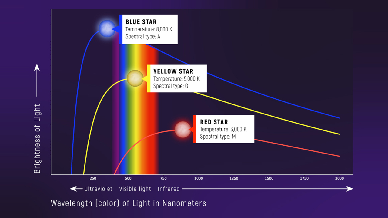
Before we write down the equation, look at the Planck curves for stars of different temperatures:
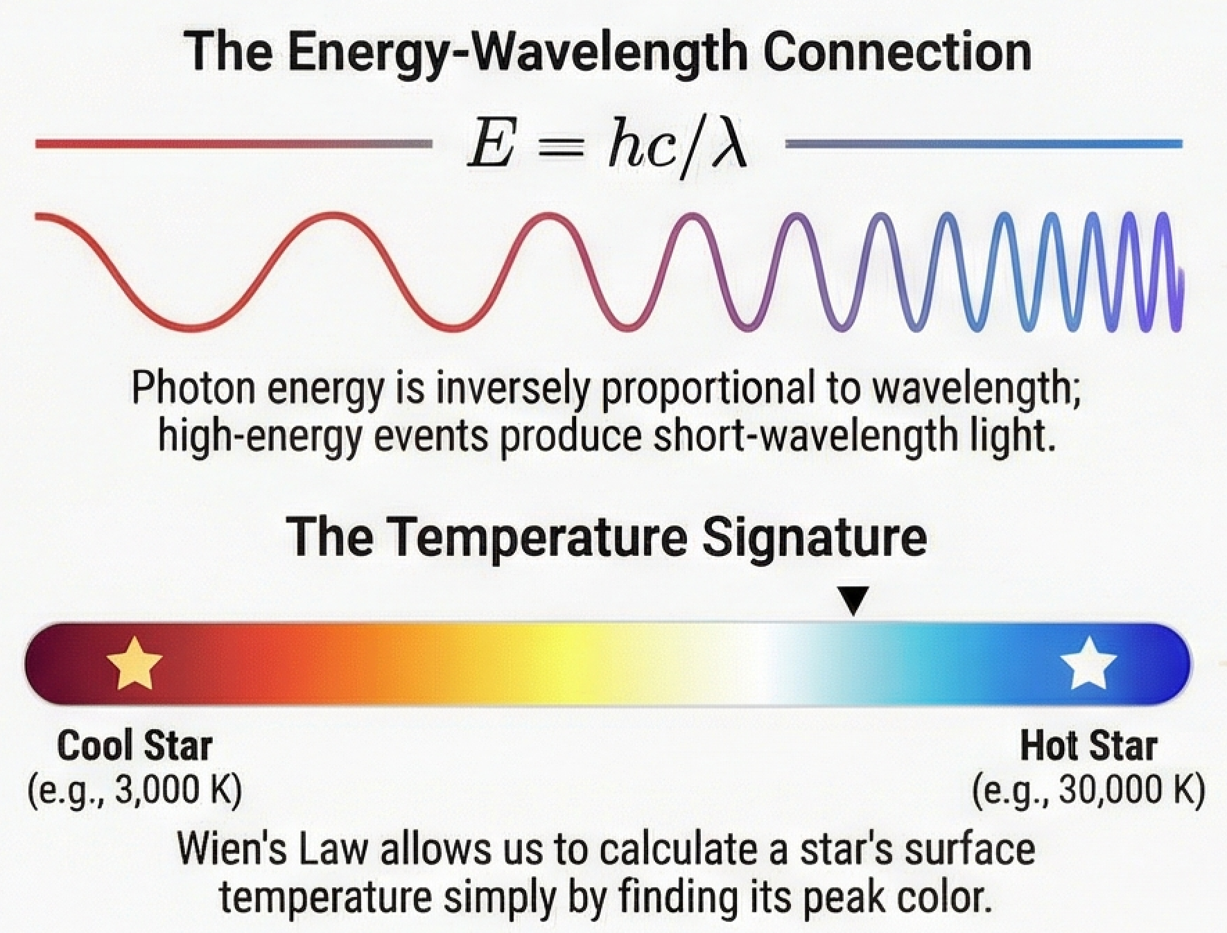
What to notice: E = hc/λ means shorter wavelength = higher energy. Wien’s Law lets us calculate temperature from color: cool stars are red (~3,000 K), hot stars are blue (~30,000 K).
Notice that each curve has a single peak, and hotter stars peak at shorter (bluer) wavelengths while cooler stars peak at longer (redder) wavelengths. Wien’s displacement law is the equation that quantifies this pattern.
Review and Quantification
From Lecture 4 (Module 1), you learned Wien’s displacement law:
\[ \lambda_{\text{peak}} = b T^{-1} \tag{3}\]
What it predicts
Given temperature \(T\), it predicts the peak wavelength \(\lambda_{\text{peak}}\) of thermal emission.
What it depends on
\(\lambda_{\text{peak}} \propto T^{-1}\).
What it’s saying
Hotter objects peak at shorter wavelengths (bluer); cooler objects peak at longer wavelengths (redder).
Assumptions
- Object radiates as a blackbody (or approximately so)
- Applies to thermal (temperature-driven) radiation
See: the equation
where \(b = 0.2898\) cm·K \(= 2.898 \times 10^{6}\) nm·K is Wien’s constant.
Units sanity check: \(b\) has units of length\(\times\)temperature, so \(b/\lambda\) has units of K.
Interpretation — Hotter means bluer; cooler means redder: - \(\lambda_{\text{peak}}\) is the wavelength where the star’s blackbody curve peaks - It depends only on temperature: hotter objects peak at shorter (bluer) wavelengths - The relationship is inverse: \(\lambda_{\text{peak}} \propto T^{-1}\)
Observable in practice: - You measure the color/spectrum and identify the peak (or use other methods to estimate the effective wavelength) - You use Wien’s law to calculate temperature - Unlike distance, which requires additional information, temperature can be read directly from color
From idealized peak to real filters: In practice, astronomers rarely measure the exact peak wavelength. Instead, they observe a star through standardized broadband filters (e.g., blue \(B\) and visual \(V\) filters) and compare the flux in each band. A star whose Planck curve peaks at short wavelengths will appear brighter through the blue filter than through the red filter. The ratio of fluxes in two filters serves as a proxy for the peak wavelength — and hence the temperature — grounded in the same Wien’s-law physics. You’ll encounter this “color index” technique formally in later lectures, but the physical principle is the one you already know: a hotter blackbody puts more of its radiation at shorter wavelengths.
The constant \(b = 2.898 \times 10^6\) nm·K applies to the peak of the per-wavelength Planck curve \(B_\lambda(T)\) — the curve you get when plotting intensity vs. wavelength. If you instead plot intensity vs. frequency (\(B_\nu(T)\)), the peak shifts to a different location because you’re stretching the axis nonlinearly. The per-frequency Wien constant is \(b_\nu \approx 5.88 \times 10^{10}\) Hz/K.
In this course we always use the per-wavelength form \(\lambda_{\text{peak}} = b/T\). If you encounter a different “peak” in another source, check which Planck function is being plotted.
From \(\lambda_{\text{peak}} = b T^{-1}\):
- If temperature doubles, peak wavelength ___?
- A star is twice as hot as the Sun. Where does it peak compared to the Sun?
- One star peaks in the red (\(\lambda \approx 700\) nm); another peaks in the blue (\(\lambda \approx 400\) nm). What’s the temperature ratio?
- Halves (\(\times 1/2\)) — peak wavelength is inversely proportional to temperature
- Halves — at twice the Sun’s temperature, peak wavelength is half the Sun’s. The Sun peaks near 500 nm, so this star would peak near 250 nm (ultraviolet).
- Blue star is \(700/400 = 1.75\times\) hotter — use the inverse relationship: if \(\lambda_1 = 700\) nm and \(\lambda_2 = 400\) nm, then \(T_1/T_2 = \lambda_2/\lambda_1 = 400/700 \approx 0.57\), so \(T_2/T_1 \approx 1.75\).
Part 5 takeaway: Wien’s law \(\lambda_{\text{peak}} = b/T\) is the tool that turns an observable (color) into a physical property (temperature). Hotter stars are bluer; cooler stars are redder. This single relationship anchors the HR diagram’s horizontal axis.
Worked Example 1: The Sun’s Temperature from Its Color
Problem: The Sun’s spectrum peaks at approximately \(\lambda_{\text{peak}} \approx 500\) nm (green-yellow light, the peak of human vision sensitivity). Calculate the Sun’s surface temperature.
Solution:
Using Wien’s displacement law: \(T = b/\lambda_{\text{peak}}\)
Step 1 — Convert units. We’re given \(\lambda_{\text{peak}} = 500\) nm. Wien’s constant is \(b = 2.898 \times 10^6\) nm·K (using the nm·K form so units match directly). Alternatively, in CGS:
\[500\ \text{nm} = 500 \times 10^{-7}\ \text{cm} = 5.00 \times 10^{-5}\ \text{cm}\]
Step 2 — Apply Wien’s law.
\[T_\odot = \frac{b}{\lambda_{\text{peak}}} = \frac{2.898 \times 10^6\ \text{nm·K}}{500\ \text{nm}} = 5796\ \text{K} \approx 5800\ \text{K}\]
\[[T] = \frac{[\text{nm·K}]}{[\text{nm}]} = \text{K}\ \checkmark\]
The nm cancels, leaving kelvins. If we had used the CGS form: \([T] = \frac{[\text{cm·K}]}{[\text{cm}]} = \text{K}\ \checkmark\)
Interpretation: Our inference matches the directly measured solar surface temperature from space-based measurements. This is not a coincidence — it’s a beautiful validation that the Sun is indeed a blackbody and that Wien’s law works.
Worked Example 2: Rigel and Betelgeuse (Temperature Contrast)
Problem: Two bright stars in Orion are visibly different colors: - Rigel (the left foot) is bright blue; peak wavelength \(\lambda_{\text{peak}} \approx 240\) nm - Betelgeuse (the right shoulder) is bright red; peak wavelength \(\lambda_{\text{peak}} \approx 830\) nm
Calculate their surface temperatures using Wien’s law.
Solution:
For Rigel:
Step 1 — Convert units (already in nm, matching our Wien’s constant): \[\lambda_{\text{peak}} = 240\ \text{nm} = 2.40 \times 10^{-5}\ \text{cm}\]
Step 2 — Apply Wien’s law: \[T_{\text{Rigel}} = \frac{2.898 \times 10^6\ \text{nm·K}}{240\ \text{nm}} = 12{,}075\ \text{K} \approx 12{,}100\ \text{K}\]
Unit check: \(\text{nm·K}/\text{nm} = \text{K}\) \(\checkmark\)
For Betelgeuse:
Step 1 — Convert units: \[\lambda_{\text{peak}} = 830\ \text{nm} = 8.30 \times 10^{-5}\ \text{cm}\]
Step 2 — Apply Wien’s law: \[T_{\text{Betelgeuse}} = \frac{2.898 \times 10^6\ \text{nm·K}}{830\ \text{nm}} = 3{,}490\ \text{K} \approx 3{,}500\ \text{K}\]
Unit check: \(\text{nm·K}/\text{nm} = \text{K}\) \(\checkmark\)
Interpretation — 3.5× hotter means a completely different Planck curve:
\[\frac{T_{\text{Rigel}}}{T_{\text{Betelgeuse}}} = \frac{12{,}100}{3{,}500} \approx 3.5\]
Rigel is about 3.5 times hotter than Betelgeuse. Their visible colors directly reflect this temperature difference: hot objects are blue, cool objects are red. This is the color-temperature relationship that will anchor the HR diagram’s horizontal axis.
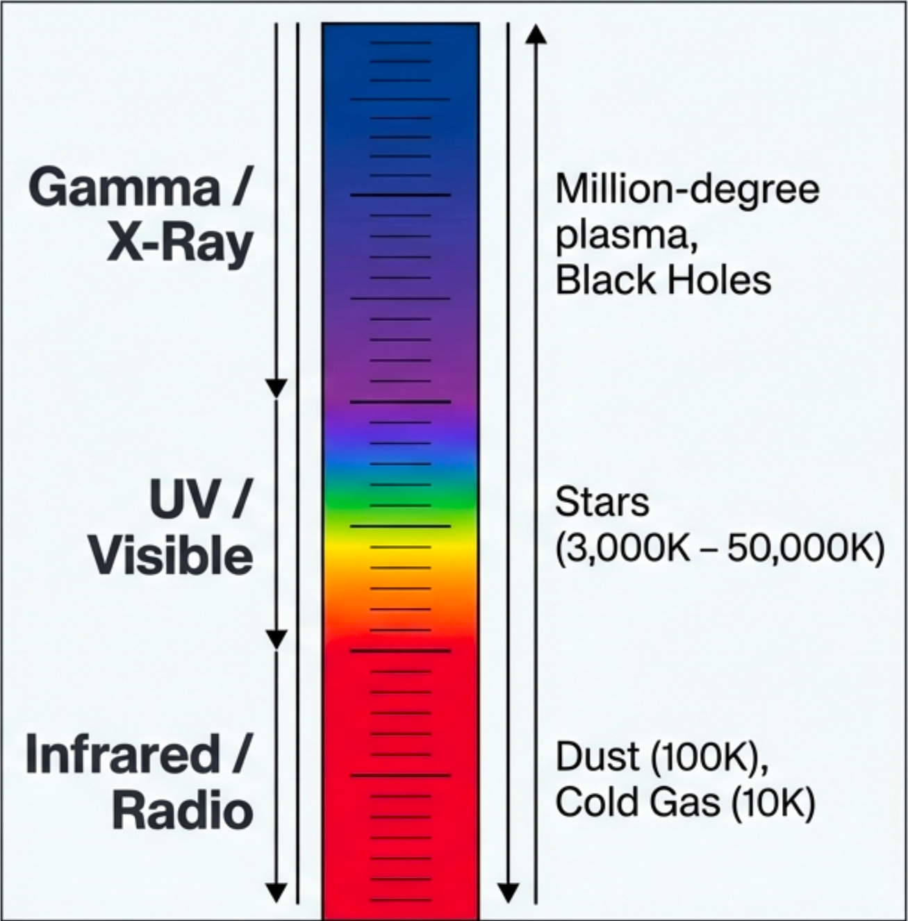
What to notice: The EM spectrum is a temperature ladder. Gamma/X-ray = million-degree plasma; UV/Visible = stellar surfaces (3,000–50,000 K); Infrared/Radio = dust and cold gas (10–100 K). (Credit: Course illustration (A. Rosen))
In Lecture 4 (Module 1), you saw the family of Planck curves \(B_\lambda(T)\) — each temperature producing a different curve shape and peak location. Rigel and Betelgeuse sit at opposite ends of that family: Rigel’s curve peaks in the ultraviolet (~240 nm) and Betelgeuse’s in the near-infrared (~830 nm). But wait — if their peaks are outside visible light, why do we see them as blue-white and deep red? Because the Planck curve is broad. Rigel’s curve peaks in the UV but its long-wavelength tail floods the visible band with more blue light than red, so we see it as blue-white. Betelgeuse’s curve peaks in the near-IR but its short-wavelength tail sends more red light than blue into the visible band, so we see it as deep red. The peak is outside our eyes’ range, but the tail still determines the visible color. Wien’s law quantifies the connection: measure the peak, know the temperature.
Check Yourself
- If a star’s peak wavelength is half the Sun’s, what is its temperature relative to the Sun?
- A star has \(\lambda_{\text{peak}} = 1.0\) \(\mu\)m. What is its temperature? (Hint: \(1.0\ \mu\text{m} = 1000\ \text{nm}\).)
- Two stars are the same luminosity but different colors. Which must have a smaller radius — the hot (blue) one or the cool (red) one? Include one equation in your justification.
Part 6: Inferring Stellar Radii
At this point, it can feel surprising that we infer a star’s radius from light measured at Earth. We trust this chain because it is cross-validated where methods overlap: nearby stars with geometric distances (parallax) match luminosities from photometry, some stellar angular diameters are measured directly with interferometry, and eclipsing binaries provide independent size constraints. Effective temperatures from spectral-energy fits and color methods also agree within expected uncertainty ranges. The chain is model-based, but it is repeatedly tested against independent observables.
When a problem feels busy, reduce it to four moves:
- Flux + distance \(\rightarrow\) luminosity (Lecture 1)
- Color or \(\lambda_{\text{peak}} \rightarrow T_{\text{eff}}\) (Wien’s law)
- Luminosity + temperature \(\rightarrow\) radius (Stefan-Boltzmann)
- Apply corrections/checks (dust reddening, bolometric corrections, uncertainty propagation)
The Complete Chain
Now you have all the pieces:
- From Lecture 1: Measure flux at Earth + measure distance → infer luminosity \(L\)
- From Lecture 4 (Module 1): Measure spectrum, find peak → apply Wien’s law → infer temperature \(T\)
- From Stefan-Boltzmann: Given \(L\) and \(T\), solve for radius \(R\).
Whenever possible, solve in solar units first:
\[\frac{R}{R_\odot} = \left(\frac{L/L_\odot}{(T/T_\odot)^4}\right)^{1/2}\]
This avoids large constants and makes sanity checks faster.
The Algebra: Isolating \(R\) (Step by Step)
Start from the Stefan-Boltzmann law:
\[L = 4\pi R^2 \sigma T^4\]
We want \(R\), so isolate \(R^2\) by dividing both sides by \(4\pi\sigma T^4\):
\[R^2 = \frac{L}{4\pi\sigma T^4}\]
Then raise both sides to the \(1/2\) power:
\[\boxed{R = \left(\frac{L}{4\pi\sigma T^4}\right)^{1/2}}\]
A common mistake is to write \(R = L/(4\pi\sigma T^4)\) — that gives \(R^2\), not \(R\). You must raise to the \(1/2\) power as the final step. Always check: does your answer have units of length (cm)?
\[[R] = \left(\frac{[\text{erg/s}]}{[\text{erg}\ \text{cm}^{-2}\ \text{s}^{-1}\ \text{K}^{-4}] \times [\text{K}^4]}\right)^{1/2} = \left(\frac{\text{erg/s}}{\text{erg}\ \text{cm}^{-2}\ \text{s}^{-1}}\right)^{1/2} = (\text{cm}^2)^{1/2} = \text{cm}\ \checkmark\]
In solar units (often easier): apply the same algebra to the dimensionless ratio \(L/L_\odot = (R/R_\odot)^2 (T/T_\odot)^4\), isolating \((R/R_\odot)^2\):
\[\left(\frac{R}{R_\odot}\right)^2 = \frac{L/L_\odot}{(T/T_\odot)^4} \quad \Longrightarrow \quad \frac{R}{R_\odot} = \left(\frac{L/L_\odot}{(T/T_\odot)^4}\right)^{1/2}\]
This is the observational technique that revealed stellar sizes before spectroscopic interferometry — and no physical constants appear in the solar-unit form.
Part 6 takeaway: Solving Stefan-Boltzmann for radius requires isolating \(R^2\) first, then raising to the \(1/2\) power. The solar-unit form eliminates all physical constants and reduces the problem to ratios.
In Lecture 1, you measured distance and luminosity. In Lecture 4 (Module 1), color gave you temperature. Now Stefan-Boltzmann completes the triangle: \(L\), \(T\), and \(R\) are connected by a single equation, so knowing any two determines the third. Every star in the sky is characterized by just three numbers — and you can infer all three from two measurements (brightness + color) and one distance.
Problem: Sirius A (the brightest star in the night sky) has: - Luminosity: \(L_{\text{Sirius}} \approx 25 L_\odot\) - Temperature: \(T_{\text{Sirius}} \approx 9{,}900\) K (from color) - Solar values: \(T_\odot = 5800\) K, \(R_\odot = 6.96 \times 10^{10}\) cm
Calculate Sirius A’s radius.
Solution:
Using the solar-unit form:
\[\frac{R_{\text{Sirius}}}{R_\odot} = \left(\frac{L_{\text{Sirius}}/L_\odot}{(T_{\text{Sirius}}/T_\odot)^4}\right)^{1/2}\]
Step 1 — Calculate the temperature ratio: \[\frac{T_{\text{Sirius}}}{T_\odot} = \frac{9{,}900\ \text{K}}{5{,}800\ \text{K}} = 1.707\]
(Units: K/K = dimensionless \(\checkmark\))
Step 2 — Raise to the fourth power: \[(T_{\text{Sirius}}/T_\odot)^4 = (1.707)^4 = 1.707^2 \times 1.707^2 = 2.914 \times 2.914 \approx 8.49\]
Step 3 — Compute \((R/R_\odot)^2\): \[\left(\frac{R_{\text{Sirius}}}{R_\odot}\right)^2 = \frac{25}{8.49} = 2.94\]
Step 4 — Raise to the \(1/2\) power to get \(R/R_\odot\): \[\frac{R_{\text{Sirius}}}{R_\odot} = (2.94)^{1/2} \approx 1.71\]
So Sirius A’s radius is approximately \(1.7\,R_\odot\).
Step 5 — Convert to physical units: \[R_{\text{Sirius}} \approx 1.71 \times R_\odot = 1.71 \times 6.96 \times 10^{10}\ \text{cm} = 1.19 \times 10^{11}\ \text{cm}\]
Converting cm to km (\(1\ \text{km} = 10^5\ \text{cm}\)): \[R_{\text{Sirius}} = \frac{1.19 \times 10^{11}\ \text{cm}}{10^5\ \text{cm/km}} = 1.19 \times 10^{6}\ \text{km} \approx 1{,}190{,}000\ \text{km}\]
Compare to the Sun: \(R_\odot \approx 696{,}000\) km.
Interpretation — Hot stars don’t need to be big to be bright: Sirius A is a hot, luminous A-type star, but it’s only about 70% larger than the Sun despite being 25 times brighter. The high temperature (\(T_{\text{Sirius}} \approx 1.7\,T_\odot\)) means each square centimeter radiates \((1.707)^4 \approx 8.5\) times more power than the Sun’s surface, so it doesn’t need to be enormous.
Before you work through the next example, commit to a prediction. Betelgeuse is \(10^5\) times more luminous than the Sun but only 60% as hot. Will its radius be closer to 10×, 100×, or 1000× the Sun’s? Write down your guess and your reasoning — then check it against the calculation below.
Worked Example 4: Betelgeuse (A Supergiant)
Problem: Betelgeuse (the red supergiant in Orion) has: - Luminosity: \(L_{\text{Betelgeuse}} \approx 10^5 L_\odot\) (100,000 times the Sun) - Temperature: \(T_{\text{Betelgeuse}} \approx 3{,}500\) K (from color)
Calculate Betelgeuse’s radius and compare it to the Sun.
Solution:
Using the solar-unit form:
\[\frac{R_{\text{Betelgeuse}}}{R_\odot} = \left(\frac{L_{\text{Betelgeuse}}/L_\odot}{(T_{\text{Betelgeuse}}/T_\odot)^4}\right)^{1/2}\]
Step 1 — Calculate the temperature ratio: \[\frac{T_{\text{Betelgeuse}}}{T_\odot} = \frac{3{,}500\ \text{K}}{5{,}800\ \text{K}} = 0.6034\]
(Units: K/K = dimensionless \(\checkmark\))
Step 2 — Raise to the fourth power: \[(T_{\text{Betelgeuse}}/T_\odot)^4 = (0.6034)^4 = 0.6034^2 \times 0.6034^2 = 0.3641 \times 0.3641 \approx 0.1326\]
Step 3 — Compute \((R/R_\odot)^2\): \[\left(\frac{R_{\text{Betelgeuse}}}{R_\odot}\right)^2 = \frac{10^5}{0.1326} = 7.54 \times 10^5\]
Step 4 — Raise to the \(1/2\) power to get \(R/R_\odot\): \[\frac{R_{\text{Betelgeuse}}}{R_\odot} = (7.54 \times 10^5)^{1/2} = (7.54)^{1/2} \times (10^5)^{1/2} = 2.75 \times 316 \approx 868\]
So Betelgeuse’s radius is approximately \(870\,R_\odot\).
Step 5 — Convert to physical units: \[R_{\text{Betelgeuse}} \approx 870 \times R_\odot = 870 \times 6.96 \times 10^{10}\ \text{cm} = 6.06 \times 10^{13}\ \text{cm}\]
Converting cm to km (\(1\ \text{km} = 10^5\ \text{cm}\)): \[R_{\text{Betelgeuse}} = \frac{6.06 \times 10^{13}\ \text{cm}}{10^5\ \text{cm/km}} = 6.06 \times 10^{8}\ \text{km} \approx 606{,}000{,}000\ \text{km}\]
Converting km to AU (\(1\ \text{AU} = 1.496 \times 10^8\ \text{km}\)): \[R_{\text{Betelgeuse}} = \frac{6.06 \times 10^8\ \text{km}}{1.496 \times 10^8\ \text{km/AU}} \approx 4.1\ \text{AU}\]
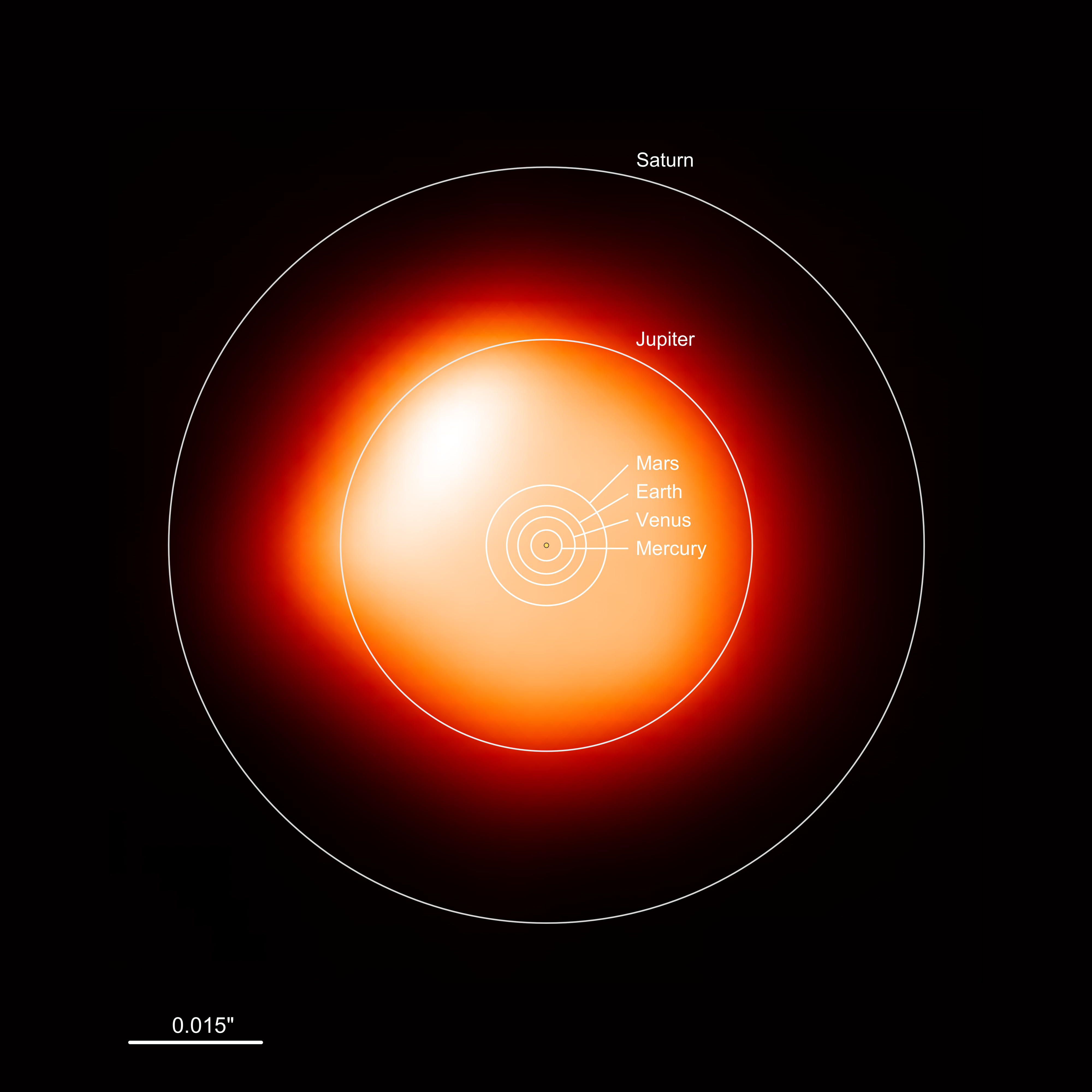
What to notice: Betelgeuse is HUGE — it would engulf Mercury, Venus, Earth, and Mars, and extend to about 4 AU, approaching but not quite reaching Jupiter’s orbit (5.2 AU). Red supergiants are cool (~3,500 K) but luminous because of their enormous surface area. (Credit: ESO/L. Calçada)
Comparison: If you placed Betelgeuse at the center of our solar system, its surface would extend to about 4 AU — past the orbit of Mars (1.5 AU) and approaching Jupiter (5.2 AU). The Sun, by comparison, fits comfortably in the inner solar system at a radius of only \(0.005\) AU.
Why so enormous? — Cool surface means huge area to compensate. Betelgeuse is much cooler than the Sun (\(T_{\text{Betelgeuse}} \approx 0.6\,T_\odot\)), so each square centimeter of its surface radiates only \((0.603)^4 \approx 0.13\) times as much power as the Sun’s. But Betelgeuse is \(10^5\) times more luminous. To produce that much total power with so little power per unit area, the surface area must be enormous: \(\text{Area}_{\text{Betelgeuse}}/\text{Area}_\odot = (870)^2 \approx 7.6 \times 10^5\). Betelgeuse has roughly 760,000 times the Sun’s surface area.
Check Yourself
- Two stars have the same luminosity. If one is twice as hot as the other, which is larger? By what factor? (Hint: \(R \propto T^{-2}\) at fixed \(L\).)
- Betelgeuse is much cooler than the Sun but 100,000 times more luminous. Explain this using Stefan-Boltzmann.
- If a star’s temperature is unknown, can you determine its radius from luminosity alone?
Part 7: Color and the HR Diagram (Preview)
The Temperature-Color Connection
You now know: - Hot stars are blue (short peak wavelength, high \(T\)) - Cool stars are red (long peak wavelength, low \(T\)) - The relationship is quantitative: \(\lambda_{\text{peak}} = b T^{-1}\)
In practice, astronomers use “color indices” — comparing a star’s brightness in two different wavelength bands (e.g., blue vs. red filters) — to estimate temperature without finding the exact peak wavelength. The physics is the same: color maps to temperature.
In 1911, the Danish chemist Ejnar Hertzsprung plotted the brightness of stars in the Pleiades cluster against their color and noticed that most fell along a diagonal band — what we now call the main sequence. Independently, the American astronomer Henry Norris Russell produced a similar diagram in 1913 using nearby stars with known parallax distances, plotting absolute brightness against spectral type. Neither initially understood why stars clustered where they did — that required the Stefan-Boltzmann connection you’re learning now. The diagram that bears both their names became the single most important tool in stellar astrophysics, revealing patterns that eventually led to our understanding of stellar structure and evolution.
The HR Diagram’s Horizontal Axis
The Hertzsprung-Russell diagram plots stellar luminosity (vertical axis) versus something on the horizontal axis. Historically, it was spectral type (OBAFGKM sequence); modern versions often use temperature or color.
The key insight: the horizontal axis is a temperature axis.
- Left side: hot, blue stars (O and B types, \(T > 7{,}000\) K)
- Right side: cool, red stars (K and M types, \(T < 4{,}000\) K)
- Hot stars are on the left; cool stars are on the right (historical convention from spectral classification)
The stellar spectral sequence OBAFGKM, defined by prominent spectral lines (ionized helium, hydrogen Balmer lines, metal absorption, etc.), is fundamentally sorted by temperature:
| Type | Temperature Range | Color | Example |
|---|---|---|---|
| O | 30,000–50,000 K | Blue-UV | \(\theta\) Orionis |
| B | 10,000–30,000 K | Blue-white | Rigel, Spica |
| A | 7,000–10,000 K | White | Vega, Sirius |
| F | 6,000–7,500 K | Yellow-white | Procyon A |
| G | 5,200–6,000 K | Yellow | Sun |
| K | 3,700–5,200 K | Orange | Aldebaran |
| M | <3,700 K | Red | Betelgeuse, Proxima Cen |
Why the spectral lines change is a matter of ionization equilibrium (which ions exist at a given temperature) and which atomic transitions can be excited — this will be covered in Module 2’s later lectures on spectroscopy. But the fundamental fact is clear: later spectral type = cooler temperature.
Lines of Constant Radius on the HR Diagram
Since \(L \propto R^2 T^4\) (Stefan-Boltzmann), for a fixed radius \(R\), luminosity varies as \(T^4\). This means: - Stars with the same radius lie on a curve in the HR diagram - The curve is steep (luminosity scales as \(T^4\), so hot stars at fixed \(R\) are much more luminous than cool stars) - In Lecture 6, you’ll see how these “evolutionary tracks” shape the HR diagram
For now, the key point: every star you can observe lies on some curve of constant \(R\) in the HR-diagram plane.
Preview of the HR Diagram Structure
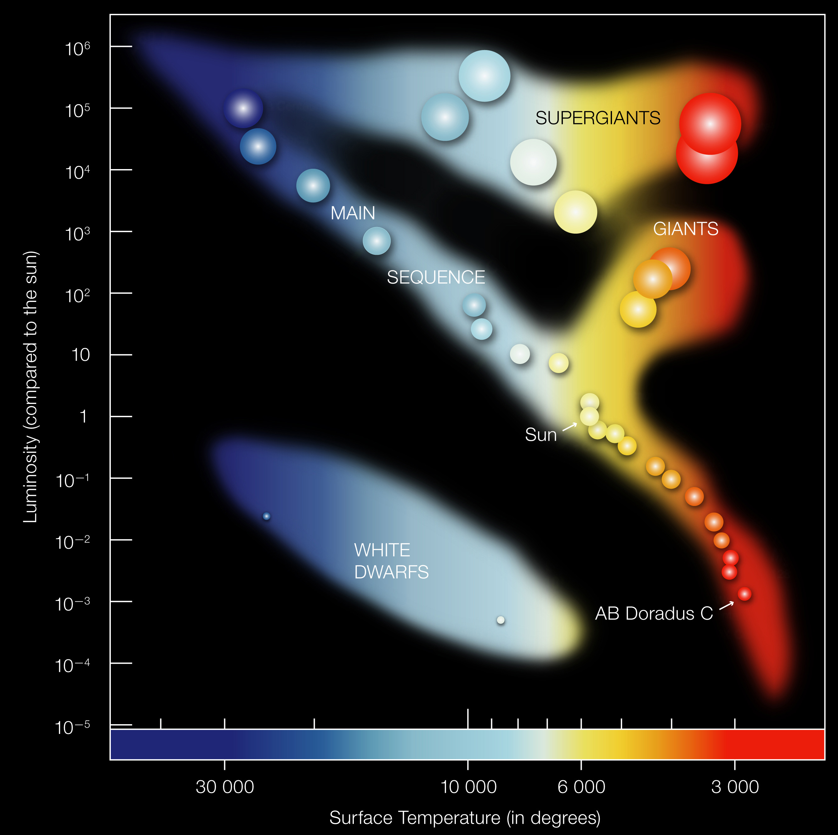
What to notice: The H-R diagram separates stars into main sequence, giants/supergiants, and white dwarfs; temperature decreases left-to-right while luminosity increases upward. (Credit: ESO)
When you plot many stars on the HR diagram, they don’t scatter uniformly. Instead, they cluster in distinct regions:
- Main sequence (diagonal band from hot/luminous to cool/dim): stars burning hydrogen in their cores, where the Sun lives. Most stars spend most of their lives here.
- Giant branch (cool but very luminous — upper right): evolved stars with greatly expanded envelopes. Their large radii (\(R \gg R_\odot\)) compensate for their lower temperatures. Betelgeuse lives here.
- White dwarf sequence (hot but very dim — lower left): stellar remnants about the size of Earth. Their tiny radii (\(R \sim 0.01\,R_\odot\)) explain why they’re faint despite high surface temperatures.
Each region corresponds to a different physical state of stellar structure — but the Stefan-Boltzmann law applies to all of them. The lines of constant radius you can draw on the HR diagram separate these populations: main-sequence stars occupy a band near \(R \sim 0.1\)–\(10\,R_\odot\), giants extend to hundreds of \(R_\odot\), and white dwarfs cluster near \(0.01\,R_\odot\). Your ability to measure colors and brightness and infer sizes is what makes the HR diagram not just a pretty plot, but a diagnostic tool for understanding stellar evolution. In Lecture 3, we’ll learn how spectral lines refine temperature measurements and reveal chemical composition. In Lecture 4, we’ll formalize the OBAFGKM spectral classification. And by Lecture 6, we’ll build the full HR diagram from real data and see these patterns emerge.
Part 7 takeaway: The HR diagram is organized by temperature (horizontal) and luminosity (vertical). Lines of constant radius are diagonal curves across it. Every star’s position encodes its temperature, luminosity, and radius simultaneously.
Part 8: Assumptions and Limitations
Where Stefan-Boltzmann Applies (and Where It Doesn’t)
The Stefan-Boltzmann law assumes:
- Spherical symmetry: The star radiates uniformly in all directions from a sphere of radius \(R\)
- In reality: Some stars are rapid rotators (oblate, not spherical) or have starspots; binaries can be distorted by tidal forces
- Impact: Small error for most stars; significant for rapidly rotating stars or eclipsing binaries
- Uniform surface temperature: All parts of the surface are at the same temperature \(T\)
- In reality: Stars have temperature gradients; sunspots are cooler; stellar atmospheres have structure
- Impact: \(T\) should be interpreted as an effective temperature — the temperature a uniform blackbody would need to match the total flux
- Practical: The effective temperature \(T_\text{eff}\) from Wien’s law or other methods is the right quantity to use
- Blackbody radiation: The spectrum follows a Planck curve
- In reality: Real stars have absorption lines and non-thermal emission
- Impact: The overall Planck shape is still a good approximation; absorption lines are a second-order effect
- Practical: Wien’s law from the peak wavelength works; spectral lines refine the temperature estimate
How to Infer Effective Temperature in Practice
Astronomers determine stellar effective temperature using several methods, all based on Stefan-Boltzmann:
- From color/peak wavelength: Wien’s law (simplest, uses one wavelength)
- From spectral energy distribution (SED): Fit the entire spectrum to a Planck curve (more data, more robust)
- From spectroscopic features: The strength of temperature-sensitive lines (e.g., hydrogen Balmer lines, ionization balance) — requires understanding atomic physics
What to notice: A real stellar spectrum combines continuous (blackbody) shape with absorption lines. The overall curve gives temperature (Wien); the lines give composition (spectroscopy). Two inference tools in one observation. (Credit: JWST/STScI)
- From stellar parallax + photometry: If you know distance \(d\), apparent magnitude \(m\), and extinction, you can construct the entire SED and fit \(T\) directly
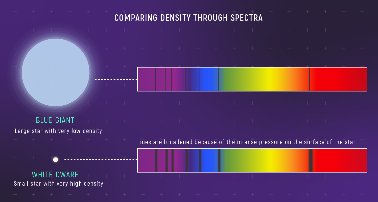
What to notice: Broader absorption lines indicate higher pressure and density, so white dwarfs show pressure-broadened spectra compared with low-density giants. (Credit: JWST/STScI)
These methods often agree to within 100–200 K, which is sufficient for most purposes.
All of the temperature and luminosity inferences above assume you’re measuring the total (bolometric) flux — integrated over all wavelengths. In practice, telescopes observe in limited wavelength bands (e.g., optical \(V\)-band), so a bolometric correction is needed to convert band-limited measurements to total luminosity. Additionally, interstellar dust absorbs and scatters starlight (extinction), preferentially removing blue light and making stars appear redder and dimmer than they truly are.
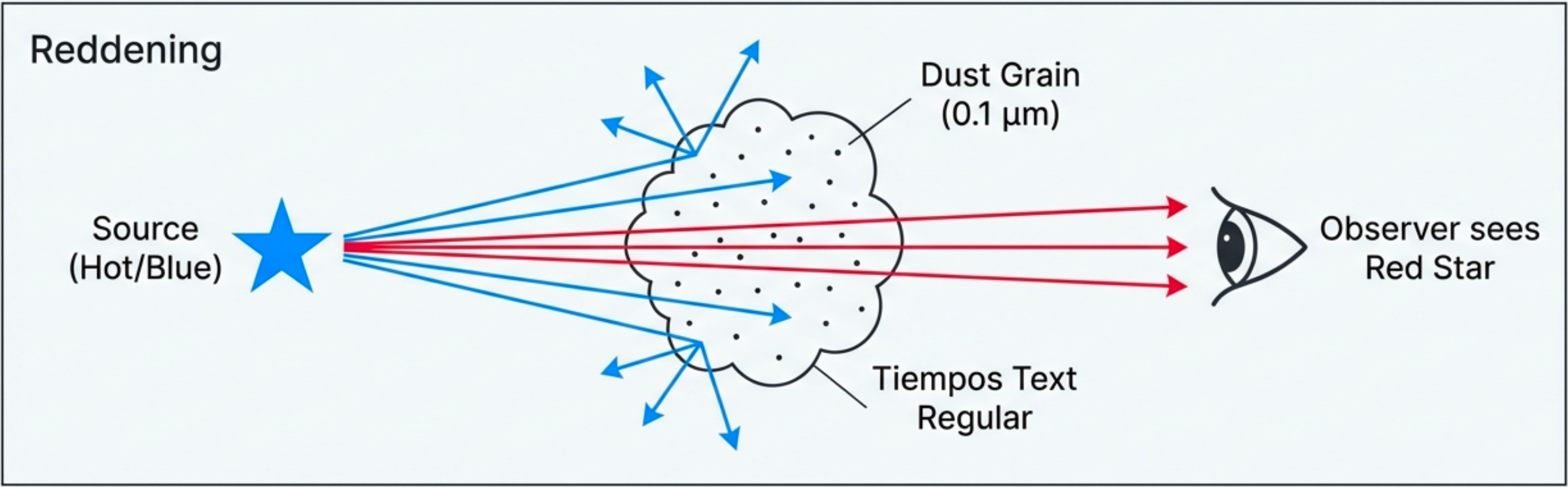
What to notice: Dust preferentially scatters blue light, making distant stars appear redder than they truly are. This ‘reddening’ must be corrected before inferring temperatures. (Credit: Course illustration (A. Rosen))
Both effects must be corrected before inferring temperatures and luminosities. The extinction problem is explored in Practice Problem 12.
Part 8 takeaway: The Stefan-Boltzmann approach works remarkably well for most stars, but the temperature we infer is an effective temperature, and real observations require bolometric corrections and extinction corrections before the inference chain is reliable.
Summary: Observable → Model → Inference
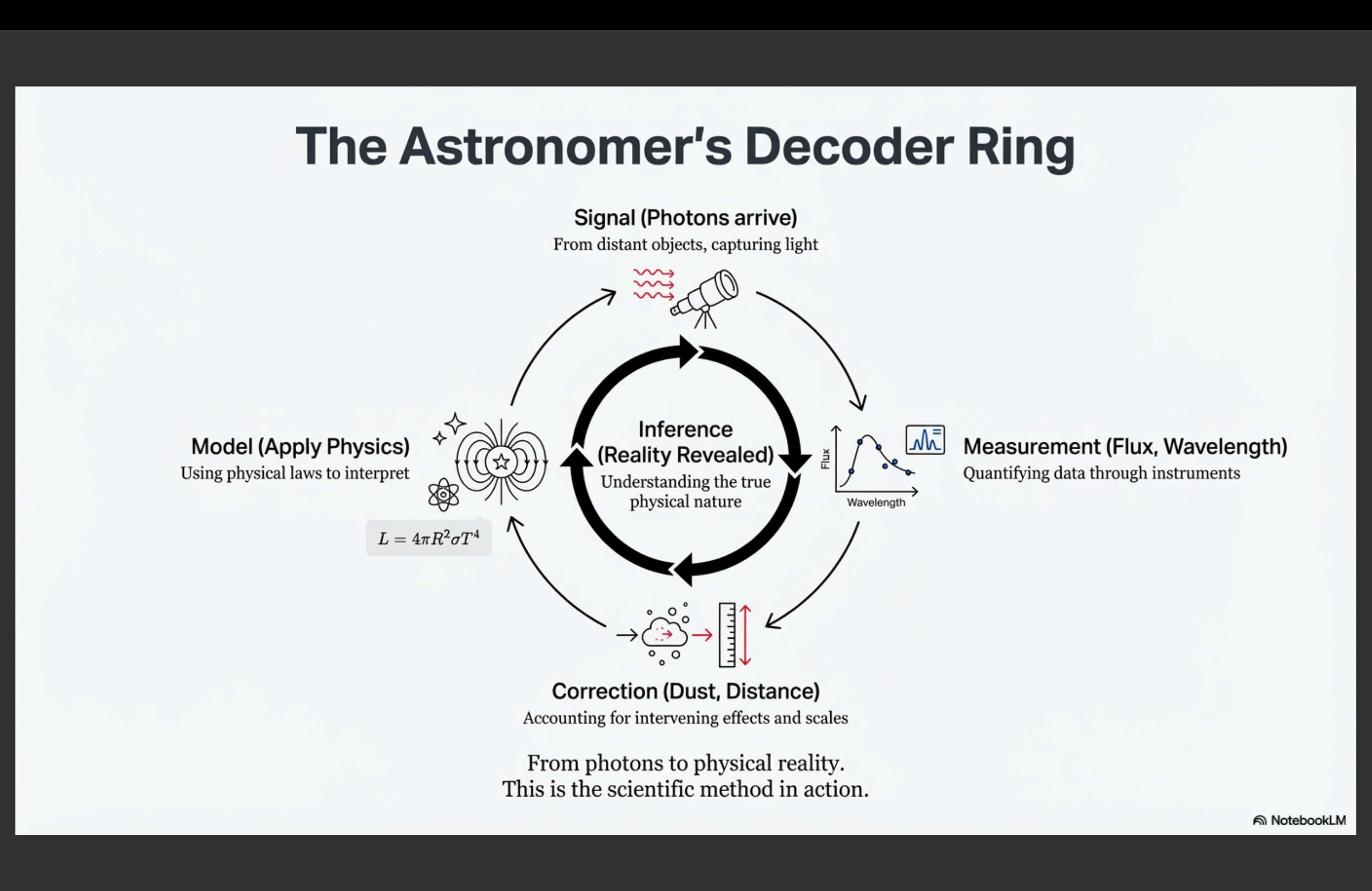
What to notice: The cycle that makes astronomy a science: Signal → Measurement → Model → Inference → Correction → back to Model. Failed predictions drive model revision. (Credit: Course illustration (A. Rosen))
| We observe | We use | We infer |
|---|---|---|
| Received flux \(F\) at distance \(d\) (Lecture 1) | \(L = 4\pi d^2 F\) | Luminosity |
| Spectrum peak wavelength \(\lambda_{\text{peak}}\) | Wien’s law: \(T = b/\lambda_{\text{peak}}\) | Temperature |
| Luminosity \(L\) and temperature \(T\) | Stefan-Boltzmann: \(R = \bigl(L/(4\pi\sigma T^4)\bigr)^{1/2}\) | Radius |
The complete inference chain: - Step 1: Measure brightness and distance → \(L\) - Step 2: Measure color → \(T\) - Step 3: Apply Stefan-Boltzmann → \(R\)
Each star you observe yields at least three fundamental properties (and many more if you measure lines, rotation, binarity, etc.). This is the power of multi-wavelength, multi-technique astronomy.
Self-Assessment Checklist
After working through this lecture, you should be able to:
You now have two of the HR diagram’s three axes: luminosity (from Lecture 1) and temperature/color (this lecture). In Lecture 3, we’ll see how absorption lines in stellar spectra reveal composition and refine temperature measurements — the science of spectroscopy. Lecture 4 formalizes the spectral classification system (OBAFGKM) and connects it to the temperature sequence you’ve already learned. By Lecture 6, you’ll build the full HR diagram from real data and see how the main sequence, giant branch, and white dwarf sequence emerge as natural consequences of stellar physics.
Practice Problems
Useful constants (for all problems below): \(b = 2.898 \times 10^6\) nm·K \(= 0.2898\) cm·K, \(\;\sigma = 5.67 \times 10^{-5}\) erg cm\(^{-2}\) s\(^{-1}\) K\(^{-4}\), \(\;1\) pc \(= 3.086 \times 10^{18}\) cm, \(\;L_\odot = 3.828 \times 10^{33}\) erg/s, \(\;T_\odot = 5800\) K, \(\;R_\odot = 6.96 \times 10^{10}\) cm \(\approx 696{,}000\) km, \(\;1\) km \(= 10^5\) cm.
Conceptual
- ⭐ Two stars, same luminosity, different colors. Star A is blue; Star B is red. Both have the same luminosity (same total power output).
- Which star has the higher effective temperature?
- Which star must have the larger radius? Explain using Stefan-Boltzmann (\(L = 4\pi R^2 \sigma T^4\)).
- If you could stand on each star’s surface (without burning up), which surface would radiate more power per square centimeter? How do you know?
- ⭐ Why Betelgeuse is huge. Betelgeuse has:
- Luminosity: \(\sim 10^5 L_\odot\) (100,000 times the Sun)
- Temperature: \(\sim 3{,}500\) K (about 60% of the Sun’s temperature)
- ⭐⭐ Peak wavelength, temperature, and radius. A star’s spectrum peaks at \(\lambda_{\text{peak}} = 1000\) nm (near-infrared), while the Sun peaks at \(\lambda_{\text{peak}} = 500\) nm.
- Is this star hotter or cooler than the Sun? By what factor? (Use Wien’s law as a ratio: \(T_{\text{star}}/T_\odot = \lambda_{\text{peak},\odot}/\lambda_{\text{peak,star}}\).)
- If this star has the same luminosity as the Sun, which must have the larger radius? By what factor? (Use \(R \propto T^{-2}\) at fixed \(L\).)
- Which star has the greater surface flux (\(F_* = \sigma T^4\))? By what factor?
- ⭐⭐ Surface brightness independence. Explain why you cannot determine a star’s distance just by measuring how bright its disk appears per unit solid angle, using the fact that surface brightness \(\text{SB} = F/\Omega\) is independent of distance. Does this principle apply most directly to unresolved point sources or to resolved objects (disks, galaxies, nebulae)?
Calculation
- ⭐ Sun’s effective temperature from Wien’s law. The Sun’s spectrum peaks at \(\lambda_{\text{peak}} = 500\) nm.
- Convert 500 nm to cm. (\(1\ \text{nm} = 10^{-7}\ \text{cm}\), so \(500\ \text{nm} = 500 \times 10^{-7}\ \text{cm} = 5.0 \times 10^{-5}\ \text{cm}\).)
- Use Wien’s law (\(T = b/\lambda_{\text{peak}}\)) with \(b = 0.2898\) cm·K to calculate the Sun’s effective temperature \(T_\odot\). Show the unit cancellation explicitly.
- Compare your answer to the known value of 5800 K.
- ⭐ Stellar temperature from color. A star’s spectrum peaks at 700 nm (red).
- Calculate its effective temperature using Wien’s law. Show the unit conversion from nm to cm (or use \(b = 2.898 \times 10^6\) nm·K directly).
- Is this star hotter or cooler than the Sun? By what factor?
- ⭐⭐ From received flux to luminosity. A star at a parallax-measured distance of \(d = 10\) pc has a measured bolometric flux at Earth of \(F = 8.0 \times 10^{-6}\) erg s\(^{-1}\) cm\(^{-2}\).
- Convert the distance to cm: \(d = 10\ \text{pc} \times 3.086 \times 10^{18}\ \text{cm/pc} = {?}\)
- Calculate the luminosity using \(L = 4\pi d^2 F\). Show units at every step to verify you get erg/s.
- Express your answer in solar luminosities (\(L/L_\odot\)). Does this luminosity remind you of any star from the worked examples?
⭐⭐ Stellar radius from Stefan-Boltzmann (ratio method). A star has:
- Luminosity: \(L = 4 L_\odot\)
- Temperature: \(T = 2 T_\odot\) (from its color)
Using the solar-unit form of Stefan-Boltzmann: \[\frac{L}{L_\odot} = \left(\frac{R}{R_\odot}\right)^2 \left(\frac{T}{T_\odot}\right)^4\]
- Show that \((R/R_\odot)^2 = (L/L_\odot) \div (T/T_\odot)^4 = 4/16 = 0.25\).
- Raise to the \(1/2\) power: \(R/R_\odot = (0.25)^{1/2} = {?}\)
- Is this star larger or smaller than the Sun? Convert to km.
- ⭐⭐ Rigel’s radius (full calculation). Rigel (a blue supergiant) has:
- Luminosity: \(L_{\text{Rigel}} = 120{,}000\,L_\odot\) (inferred from parallax + received flux)
- Effective temperature: \(T_{\text{Rigel}} = 12{,}100\) K (inferred from color via Wien’s law)
- Compute the temperature ratio \(T_{\text{Rigel}}/T_\odot\) and verify it is dimensionless.
- Raise to the fourth power: \((T_{\text{Rigel}}/T_\odot)^4 = {?}\)
- Compute \((R_{\text{Rigel}}/R_\odot)^2\), then raise to the \(1/2\) power to find \(R_{\text{Rigel}}/R_\odot\).
- Express \(R_{\text{Rigel}}\) in km. (Convert from solar radii using \(R_\odot = 6.96 \times 10^{10}\) cm and \(1\ \text{km} = 10^5\) cm.)
- How does Rigel compare to Betelgeuse (\(R_{\text{Betelgeuse}} \approx 870\,R_\odot\))? Both are supergiants — why is one so much larger?
Synthesis
⭐⭐ Complete inference chain: From photons to radius. You observe a nearby red giant with the following measurements:
- Bolometric flux received at Earth: \(F = 1.28 \times 10^{-6}\) erg s\(^{-1}\) cm\(^{-2}\)
- Peak wavelength of its spectrum: \(\lambda_{\text{peak}} = 1{,}000\) nm (near-infrared)
- Distance from parallax: \(d = 50\) pc
Walk through the full Observable → Model → Inference chain:
- Temperature from color. Use Wien’s law to calculate the effective temperature \(T\). Show units. Then compute \(T/T_\odot\).
- Luminosity from flux + distance. Convert \(d = 50\) pc to cm, then use \(L = 4\pi d^2 F\) to calculate the luminosity in erg/s. Show all unit conversions. Express the result as \(L/L_\odot\).
- Radius from Stefan-Boltzmann. Using the solar-unit form, first compute \((R/R_\odot)^2\), then raise to the \(1/2\) power to find \(R/R_\odot\).
- Interpret. Convert your radius to km. Is this star larger or smaller than the Sun? How does it compare to Betelgeuse (\(R \approx 870\,R_\odot\))? Does the combination of cool temperature and large radius make physical sense?
- ⭐⭐ HR Diagram reasoning. Three stars lie on the HR diagram:
- Star A: \(T = 6{,}000\) K, \(L = 1\,L_\odot\) (like the Sun)
- Star B: \(T = 3{,}000\) K, \(L = 100\,L_\odot\) (red giant)
- Star C: \(T = 12{,}000\) K, \(L = 1\,L_\odot\) (hot but dim)
- Using Stefan-Boltzmann in solar units, calculate the radius of each star in solar radii. For each star, show \((R/R_\odot)^2\) first, then raise to the \(1/2\) power.
- Which star is largest? Which is smallest?
- Sketch these three points on an HR diagram (luminosity vs. temperature, with \(T\) increasing to the left). Draw approximate lines of constant radius through each point. What do these lines tell you about the giant and white-dwarf regions of the HR diagram?
- ⭐⭐⭐ The effect of extinction on temperature inference. Interstellar dust reddens starlight by scattering blue photons more than red ones. An observer measures a star and finds:
- Observed peak wavelength: \(\lambda_{\text{obs}} = 700\) nm (appears very red)
- True peak wavelength (after correcting for dust): \(\lambda_{\text{true}} = 500\) nm
- Calculate the apparent temperature from the observed (reddened) color. Show units.
- Calculate the true temperature from the corrected color. Show units.
- By what factor does dust extinction bias the inferred temperature? (Compute \(T_{\text{apparent}}/T_{\text{true}}\).)
- If an astronomer used the reddened temperature to infer the star’s radius via Stefan-Boltzmann (at the correct luminosity), would the inferred radius be too large or too small? By what factor? (Hint: \(R \propto T^{-2}\) at fixed \(L\).)
The key equations from this reading — Stefan-Boltzmann (\(L = 4\pi R^2 \sigma T^4\)), Wien’s law (\(\lambda_{\text{peak}} = b/T\)), and the flux-luminosity-distance relation (\(F = L/4\pi d^2\)) — will be provided on your formula sheet for exams and homework. You do not need to memorize them. What you do need is the ability to use them: set up the problem, identify knowns and unknowns, solve algebraically, track units, and interpret your answer physically.
Key Equations Reference
| Equation | Use | Notes |
|---|---|---|
| \(F = L/(4\pi d^2)\) | Received flux (from Lecture 1) | Distance-dependent |
| \(F_* = L/(4\pi R^2)\) | Surface flux | Star property only |
| \(F/F_* = R^2/d^2\) | Connects received and surface flux | Pure geometry |
| \(L = 4\pi R^2 \sigma T^4\) | Stefan-Boltzmann law | Connects \(L\), \(T\), \(R\) |
| \(\sigma = 5.67 \times 10^{-5}\) erg cm\(^{-2}\) s\(^{-1}\) K\(^{-4}\) | Stefan-Boltzmann constant | Memorize or reference |
| \(\lambda_{\text{peak}} = b T^{-1}\) | Wien’s displacement law (from Lecture 4 (Module 1)) | \(b = 0.2898\) cm·K; per-\(\lambda\) peak |
| \(R = \bigl(L/(4\pi\sigma T^4)\bigr)^{1/2}\) | Solve Stefan-Boltzmann for \(R\) | Don’t forget the \({}^{1/2}\) power! |
| \(L/L_\odot = (R/R_\odot)^2 (T/T_\odot)^4\) | Stefan-Boltzmann in solar units | Convenient scaling |
| \(R/R_\odot = \bigl((L/L_\odot)/(T/T_\odot)^4\bigr)^{1/2}\) | Solve for radius in solar units | Show \((R/R_\odot)^2\) first, then \({}^{1/2}\) |
Key Constants
| Constant | Value | Units |
|---|---|---|
| Stefan-Boltzmann constant | \(\sigma = 5.67 \times 10^{-5}\) | erg cm\(^{-2}\) s\(^{-1}\) K\(^{-4}\) |
| Wien’s constant | \(b = 0.2898\) | cm·K (\(= 2.898 \times 10^6\) nm·K) |
| Solar temperature | \(T_\odot = 5800\) | K |
| Solar radius | \(R_\odot = 6.96 \times 10^{10}\) | cm \(\approx 696{,}000\) km |
| Solar luminosity | \(L_\odot = 3.828 \times 10^{33}\) | erg/s |
| 1 AU | \(1.496 \times 10^{13}\) | cm \(\approx 1.496 \times 10^{8}\) km |