Ages & Lifetimes

Complete lesson

What We Know and What We Do Not

By the end of this reading, you will be able to:

Identify
the three fundamental stellar timescales (dynamical, thermal, nuclear) and the physical process each describes
Estimate
the dynamical timescale from a star’s mean density
Calculate
the Kelvin-Helmholtz timescale and explain why gravity alone cannot power the Sun for billions of years
Derive
the nuclear timescale from the mass-luminosity relation and explain why massive stars live shorter lives
Describe
the Kelvin-Helmholtz controversy and how nuclear physics resolved it
Use
scaling relations to compare lifetimes ( $\tau_\text{nuc} \propto M^{-2.5}$ )
Explain
why the separation of the three timescales ( $\tau_\text{dyn} \ll \tau_\text{KH} \ll \tau_\text{nuc}$ ) is what lets us model a star as a static equilibrium structure — the assumption the rest of Module 3 is built on

Every star is a clock, and its mass sets the alarm. In Module 2 you measured stellar luminosities, temperatures, radii, and masses — the HR diagram became a familiar landscape. But a snapshot doesn’t tell you how long anything lasts. A star shining at $10^4\,L_\odot$ is burning through its fuel far faster than one at $0.1\,L_\odot$ . How much faster? What fuel? How long until it runs out? These questions demand a new kind of reasoning — timescale reasoning — and the answers launch us into the physics of stellar structure and evolution. Timescale reasoning pays off twice. The separation between these clocks is what earns us the right to model a star as a static, balanced structure — the assumption every later reading in this module leans on — and the longest clock sets how long the star can shine.

Part 1: What We Know — and What We Don’t

The HR Diagram Is a Snapshot

In Module 2 you built the Hertzsprung-Russell diagram piece by piece — distances, luminosities, temperatures, and masses for hundreds of stars. The result is a map of the stellar population: most stars on the main sequence, with giants above and white dwarfs below. But the HR diagram is a snapshot — a single frame from a movie you haven’t seen. It shows where stars are, not how they got there or where they’re going. In a star cluster, the massive stars are already gone from the main sequence (evolved into giants or exploded) while the low-mass ones still happily burn hydrogen. That difference in lifetime is the first clue that mass controls a star’s fate.

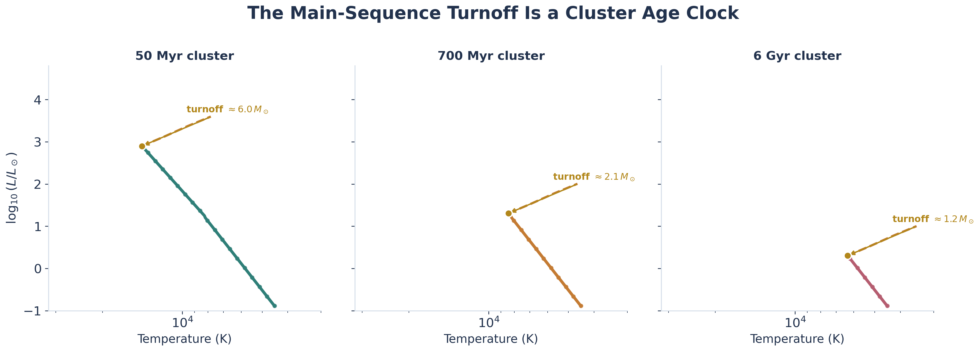
That cluster pattern is also our first age indicator. If the most massive star still on the main sequence is only about $2\,M_\odot$ , the cluster must be old enough for $10\,M_\odot$ stars to have already died. If a bright blue $10\,M_\odot$ star is still on the main sequence, the cluster is young. The observational clue is the main-sequence turnoff; this reading builds the physics that turns that clue into an age: observe a turnoff mass, map that mass to a nuclear lifetime, infer the cluster age.

Main-sequence turnoff

The point on a star cluster’s HR diagram where the most massive stars are just leaving the main sequence. Because nuclear lifetime falls steeply with mass, the turnoff mass is a clock: a high (blue) turnoff means a young cluster, a low (red) turnoff an old one.

Three-panel schematic HR-style figure for 50 Myr, 700 Myr, and 6 Gyr star clusters showing the main sequence truncated at different turnoff masses and a short evolved branch peeling away from each turnoff point. — Figure 1Coeval clusters lose their hottest, most massive main-sequence stars first. The turnoff mass moves downward with age, which is why the turnoff acts like a clock.ASTR 201 (generated)

The Module 3 Question

In Module 2 you asked: what can we measure about a star from its light? Now the deeper question:

Why does a star with mass $M$ have that particular luminosity, temperature, and radius — and how long can it last?

Answering it requires physics: what holds a star up against gravity, what generates its energy, and what happens when the source runs out. But first we need the timescales — because the first thing a physicist asks about any system is: how long does each process take?

Quick check

You know the mass-luminosity relation $L \propto M^{3.5}$ . If a star’s total fuel is proportional to its mass but its burn rate is proportional to $M^{3.5}$ , how should lifetime scale with mass?

Three Timescales That Govern a Star

Part 2: Three Timescales That Govern a Star

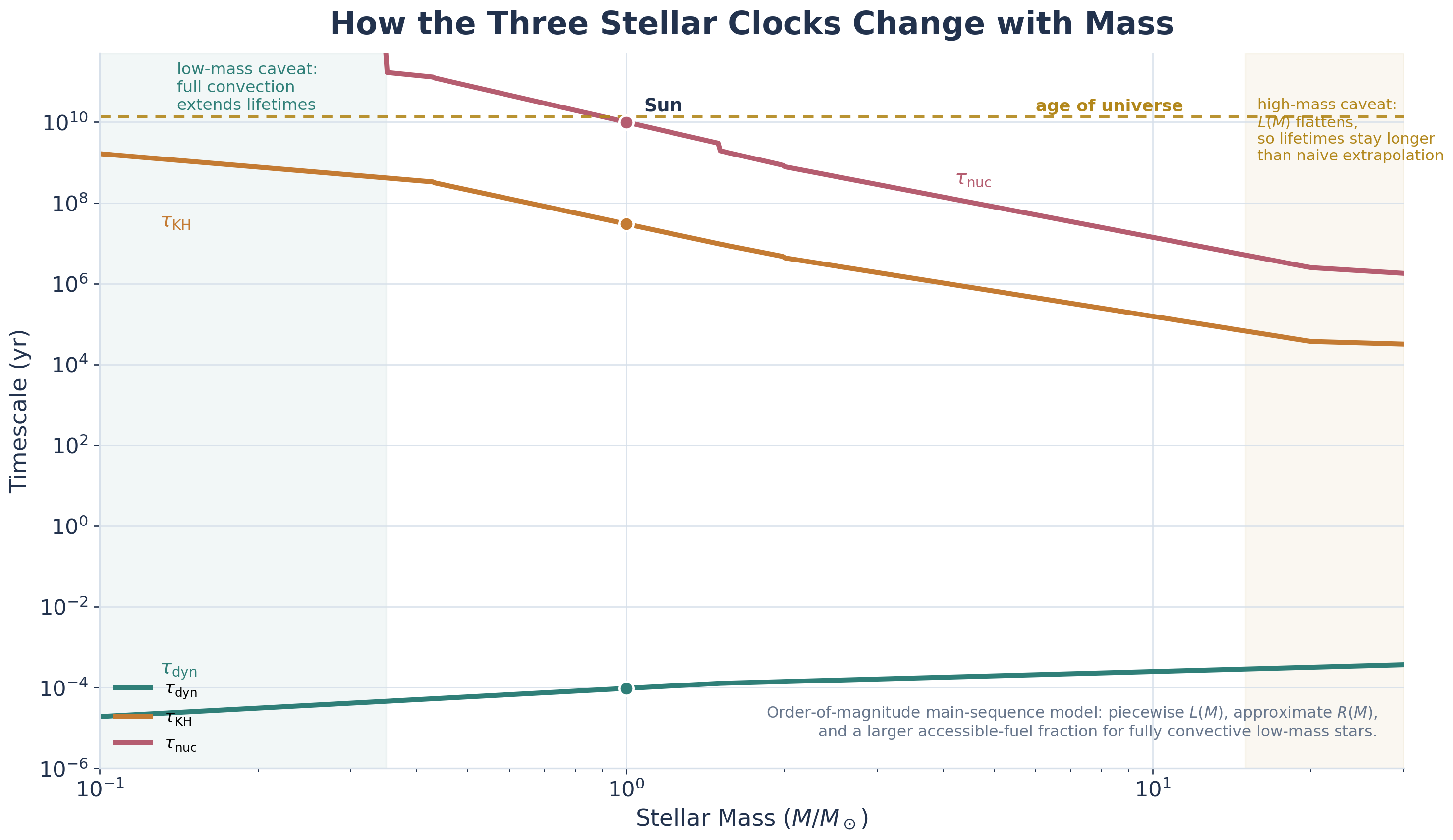
Stars are governed by three fundamental timescales, each tied to a different physical process. Their hierarchy — which is shortest, which longest — tells you what a star is doing.

Generated white-background log-log plot of stellar timescale versus stellar mass in solar units, with three labeled curves for dynamical, Kelvin-Helmholtz, and nuclear timescales, a marked Sun point, a dashed age-of-the-universe line, and shaded caveat bands at low and high mass. — Figure 2The hierarchy tau_dyn << tau_KH << tau_nuc survives across the main sequence. Massive stars still adjust quickly, but their thermal and nuclear clocks shrink drastically. Caveat bands remind us where simple scaling laws bend.ASTR 201 (generated)

Timescale	Question it answers
$\tau_\text{dyn}$	How fast would gravity rearrange the star if pressure support failed?
$\tau_\text{KH}$	How long could the star shine if gravity were its only long-term energy source?
$\tau_\text{nuc}$	How long can nuclear fusion sustain the star’s luminosity?

The Dynamical Timescale: How Fast Could a Star Collapse?

Imagine you could suddenly “turn off” all the internal pressure holding a star up. How long would it take to collapse under its own gravity? This is the dynamical timescale $\tau_\text{dyn}$ . Dimensionally, the only timescale you can build from $G$ and the mean density $\bar{\rho}$ is:

The equation is not predicting what a healthy star is doing now — it predicts how fast gravity would win if pressure support suddenly failed. (Exact free-fall calculations add numerical factors of order unity; here we keep the scaling and meaning.)

Dynamical timescale

The characteristic time for gravity to rearrange a star if pressure support failed: $\tau_\text{dyn} \sim 1/\sqrt{G\bar{\rho}}$ — about 50 minutes for the Sun. The shortest of the three stellar clocks; it sets how fast a star restores hydrostatic equilibrium after a perturbation.

Worked Example 1The Sun's Dynamical Timescale

Problem

The Sun’s mean density is $\bar{\rho}_\odot \approx 1.4~\text{g cm}^{-3}$ (about 1.4× water). Estimate its dynamical timescale.

StepEvaluate inside the square root

$G\bar{\rho}_\odot \approx (6.674 \times 10^{-8})(1.4) \approx 9.3 \times 10^{-8}~\text{s}^{-2} \Rightarrow \sqrt{G\bar{\rho}_\odot} \approx 3.1 \times 10^{-4}~\text{s}^{-1}$

StepInvert

$\tau_\text{dyn,\odot} \sim \frac{1}{3.1 \times 10^{-4}~\text{s}^{-1}} \approx 3.2 \times 10^3~\text{s} \approx 50~\text{min}$

Dimensional check

$[G\bar{\rho}] = (\text{cm}^3\text{g}^{-1}\text{s}^{-2})(\text{g cm}^{-3}) = \text{s}^{-2}$ ; the inverse square root gives seconds ✓.

Result

If pressure support were removed, the Sun would collapse in about an hour. Since it clearly is not collapsing, something holds it up — pressure. Understanding that balance is the next reading.

Problem

A white dwarf has roughly the Sun’s mass but the Earth’s radius ( $R \approx 0.009\,R_\odot$ ). Estimate its mean density and dynamical timescale. How do they compare to the Sun’s?

The Thermal (Kelvin-Helmholtz) Timescale: How Long Could Gravity Alone Power a Star?

Before anyone knew about nuclear reactions, the best guess for the Sun’s energy source was gravitational contraction — the Sun shines by slowly shrinking, converting gravitational potential energy into heat and light. Using the same grammar, $\tau \sim (\text{energy reservoir})/(\text{energy-loss rate})$ , the reservoir is the star’s gravitational binding energy: $|E| \sim GM^2/R$ (a scaling statement; a virial treatment changes only the prefactor). If there is no nuclear source, the luminosity must leak away that bound energy, $L = -dE/dt$ (the minus sign matters: a star losing energy has $dE/dt$ negative while the outward $L$ is positive). Together these give the Kelvin-Helmholtz timescale:

Here $M$ is the mass, $R$ the radius, $L$ the luminosity. The hidden assumption: this is the lifetime if gravitational contraction is the only long-term energy source.

Kelvin-Helmholtz timescale

The time a star could shine on gravitational contraction alone: $\tau_\text{KH} \sim GM^2/(RL)$ — about 30 Myr for the Sun. It is a quasi-static contraction time, not a free fall; nuclear fusion makes the real lifetime hundreds of times longer.

You can also see it from a contraction-rate argument: with $E \sim -GM^2/R$ and roughly constant mass, $dE/dt \sim (GM^2/R^2)\,dR/dt$ ; for a contracting star $dR/dt$ is negative, so $L = -dE/dt \sim (GM^2/R^2)|dR/dt|$ , giving a contraction time $R/|dR/dt| \sim GM^2/(RL) = \tau_\text{KH}$ . The Kelvin-Helmholtz timescale is not a free-fall time — it is the time for a star to contract quasi-statically as it radiates energy away.

Worked Example 2The Sun's Kelvin-Helmholtz Timescale

Problem

Estimate $\tau_\text{KH}$ for the Sun ( $M_\odot = 2.0 \times 10^{33}~\text{g}$ , $R_\odot = 7.0 \times 10^{10}~\text{cm}$ , $L_\odot = 3.8 \times 10^{33}~\text{erg/s}$ ).

StepPlug into GM²/RL

$\tau_\text{KH} \sim \frac{(6.674 \times 10^{-8})(2.0 \times 10^{33})^2}{(7.0 \times 10^{10})(3.8 \times 10^{33})} = \frac{2.67 \times 10^{59}}{2.66 \times 10^{44}}~\text{s} \approx 1.0 \times 10^{15}~\text{s}$

Dimensional check

$\dfrac{(\text{cm}^3\text{g}^{-1}\text{s}^{-2})(\text{g}^2)}{(\text{cm})(\text{erg s}^{-1})} = \dfrac{\text{erg}}{\text{erg s}^{-1}} = \text{s}$ ✓.

Result

$\tau_\text{KH} \approx 30~\text{Myr}$ . This was Lord Kelvin’s answer in the 1860s — he concluded the Sun could not be much older than 20–30 million years. Then the geologists objected.

Multiple choice

If a star has the same mass and radius as the Sun but twice the luminosity, is its Kelvin–Helmholtz timescale longer or shorter?

LongerShorter

The Kelvin-Helmholtz Controversy

Part 3: The Great Controversy — Lord Kelvin vs. The Geologists

In the late 19th century, Lord Kelvin (William Thomson) — one of the most respected physicists alive — calculated the Sun’s age from the best physics available: $\tau_\text{KH} \approx 20\text{–}30~\text{Myr}$ . But geologists had a problem. Darwin’s theory of evolution needed hundreds of millions of years, and geologists studying rock layers, erosion, and sedimentation had independently concluded the Earth was at least hundreds of millions of years old, possibly billions. Kelvin’s response was blunt: the physics was clear, so the geologists were wrong. He even argued Darwin’s theory must be flawed for lack of time.

Kelvin was wrong — but not because his physics was wrong. His calculation was perfectly correct given his assumptions. This is a useful warning: correct math does not guarantee a complete model. Kelvin assumed gravitational contraction was the Sun’s only energy source. He couldn’t know there was a far more efficient source: nuclear fusion. The resolution came in the early 20th century — radioactivity (1896), Einstein’s $E = mc^2$ (1905), Eddington’s stellar-energy proposal (1920s), and Bethe’s proton-proton chain (late 1930s). Fusion converts about $0.7\%$ of hydrogen’s rest-mass energy to radiation, and that $0.7\%$ of $Mc^2$ is enormous compared to the gravitational energy $GM^2/R$ .

Deep Dive: Enrichment: The Ratio That Changed Everything

How much more energy is available from core hydrogen fusion than from gravitational contraction? Compare the reservoirs:

$\frac{E_\text{nuc}}{E_\text{grav}} \sim \frac{\varepsilon f_M M c^2}{GM^2/R} = \frac{\varepsilon f_M c^2 R}{GM}$

Here $f_M M$ is the accessible fuel mass; for a Sun-like star $f_M \approx 0.10$ . Substituting solar values, the numerator $(0.007)(0.10)(9.0 \times 10^{20})(7.0 \times 10^{10}) \approx 4.4 \times 10^{28}~\text{cm}^3\text{s}^{-2}$ and the denominator $GM_\odot \approx 1.33 \times 10^{26}~\text{cm}^3\text{s}^{-2}$ , so

$\frac{E_\text{nuc}}{E_\text{grav}} \approx \frac{4.4 \times 10^{28}}{1.33 \times 10^{26}} \approx 3.3 \times 10^2$

(dimensionless — units cancel ✓). The accessible nuclear reservoir exceeds the gravitational one by a factor of about 300 — which is why the Sun’s nuclear lifetime ( $\sim 10~\text{Gyr}$ ) is hundreds of times longer than its Kelvin-Helmholtz timescale ( $\sim 30~\text{Myr}$ ). The fuel fraction $f_M$ varies with mass and internal mixing, so treat it as an approximate main-sequence parameter, not a universal constant. This ratio compares usable nuclear energy per unit mass to gravitational binding energy per unit mass — not the relative strengths of the forces themselves.

Quick check

Kelvin’s estimate ( $\sim 30~\text{Myr}$ ) was too short by a factor of a few hundred. What assumption was wrong, and what discovery resolved it?

The Nuclear Timescale

Part 4: The Nuclear Timescale — The True Clock

Nuclear fusion converts a fraction $\varepsilon \approx 0.007$ of hydrogen’s rest-mass energy into radiation. Only the core hydrogen participates — roughly $\sim 10\%$ of the total mass for a Sun-like star — so the accessible fuel is $f_M M$ . Dividing that reservoir by the luminosity gives the nuclear timescale:

Here $\varepsilon \approx 0.007$ is the conversion efficiency, $f_M \approx 0.10$ the accessible fuel fraction for a Sun-like star, $M$ the total mass, and $c$ the speed of light. The equation is for main-sequence hydrogen burning, and $f_M$ varies with mass and mixing.

Nuclear timescale

The time core hydrogen fusion can sustain a star’s luminosity: $\tau_\text{nuc} \sim \varepsilon f_M M c^2 / L$ — about 10 Gyr for the Sun. It is the longest of the three clocks and sets a star’s true main-sequence lifetime.

Worked Example 3The Sun's Nuclear Lifetime

Problem

Estimate the Sun’s nuclear lifetime with $\varepsilon = 0.007$ , $f_M = 0.10$ , $M_\odot = 2.0 \times 10^{33}~\text{g}$ , $c = 3.0 \times 10^{10}~\text{cm/s}$ , $L_\odot = 3.8 \times 10^{33}~\text{erg/s}$ .

StepReservoir over luminosity

$\tau_\text{nuc} \sim \frac{(0.007)(0.10)(2.0 \times 10^{33})(3.0 \times 10^{10})^2}{3.8 \times 10^{33}} = \frac{1.26 \times 10^{51}~\text{erg}}{3.8 \times 10^{33}~\text{erg/s}} \approx 3.3 \times 10^{17}~\text{s}$

Dimensional check

$\dfrac{[\text{g}][\text{cm}^2\text{s}^{-2}]}{[\text{erg s}^{-1}]} = \dfrac{[\text{erg}]}{[\text{erg s}^{-1}]} = [\text{s}]$ ✓.

Result

$\tau_\text{nuc} \approx 10~\text{Gyr}$ — about twice the Sun’s current age ( $4.6~\text{Gyr}$ ), so the Sun is roughly halfway through its hydrogen-burning life. Consistent with solar models and radiometric dating ✓.

Why Normalize to the Sun?

Rather than plug in constants every time, normalize to the Sun: write the equation for the star, write it for the Sun, and divide. The constants cancel and the answer is a dimensionless comparison to a star you know:

$\frac{\tau_\text{nuc}}{\tau_{\text{nuc},\odot}} \approx \left(\frac{\varepsilon}{\varepsilon_\odot}\right)\left(\frac{f_M}{f_{M,\odot}}\right)\left(\frac{M}{M_\odot}\right)\left(\frac{L}{L_\odot}\right)^{-1}$

For similar hydrogen-burning stars $\varepsilon$ matches (first factor 1), and for a rough comparison with similar fuel fractions this simplifies to $\tau_\text{nuc}/\tau_{\text{nuc},\odot} \approx (M/M_\odot)(L/L_\odot)^{-1}$ . A value of $0.2$ means “one-fifth of the Sun’s lifetime.” Same grammar as Kelvin-Helmholtz — reservoir over loss rate — but a nuclear reservoir.

Quick ratio example. A star with $M = 2\,M_\odot$ and $L = 10\,L_\odot$ gives $\tau_\text{nuc}/\tau_{\text{nuc},\odot} \approx 2/10 = 0.2$ , so $\tau_\text{nuc} \approx 0.2 \times 10~\text{Gyr} \approx 2~\text{Gyr}$ . Note the grammar: the scaling factor $0.2$ is dimensionless, and units appear only at the end.

The Scaling That Explains Everything

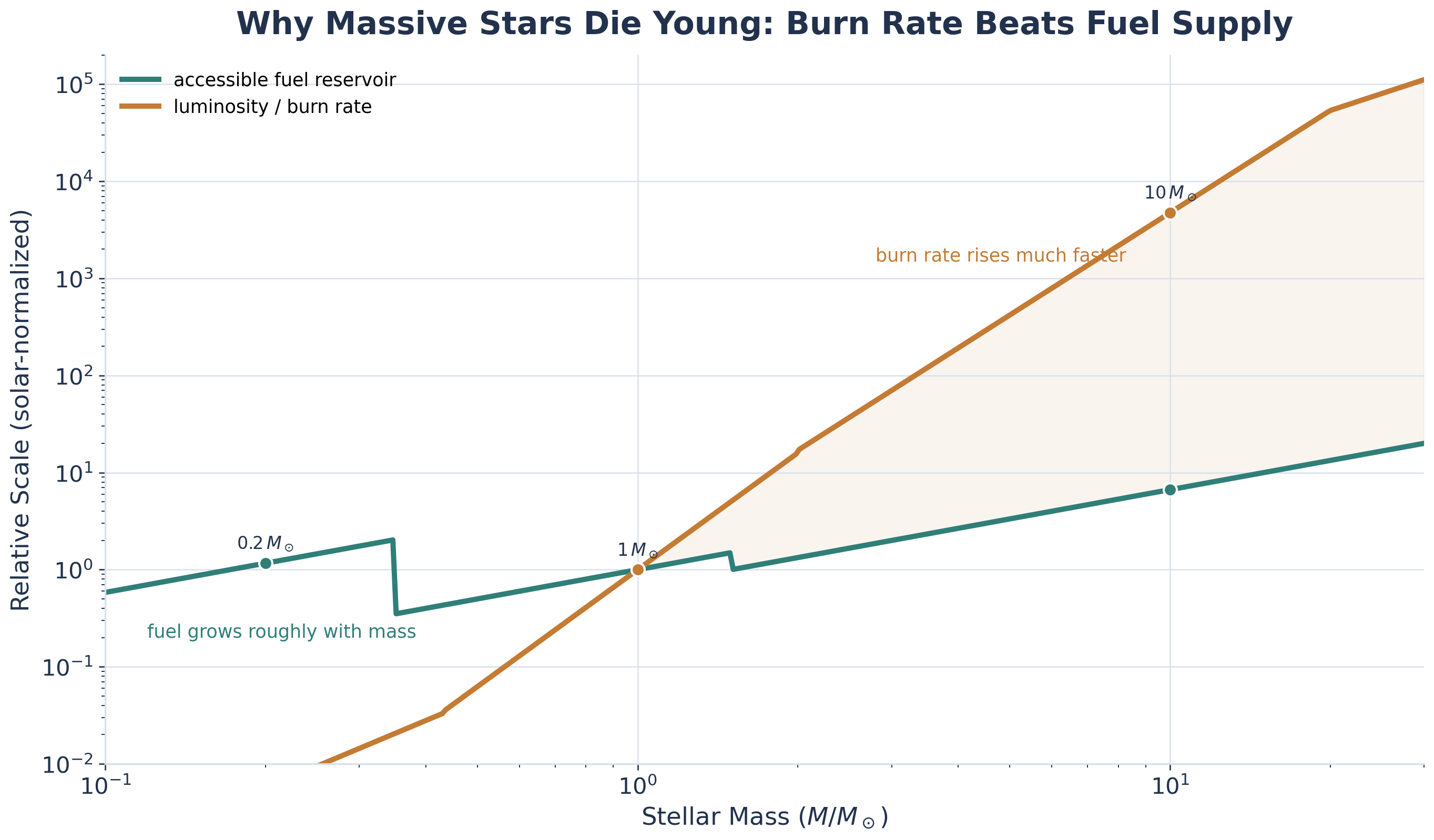
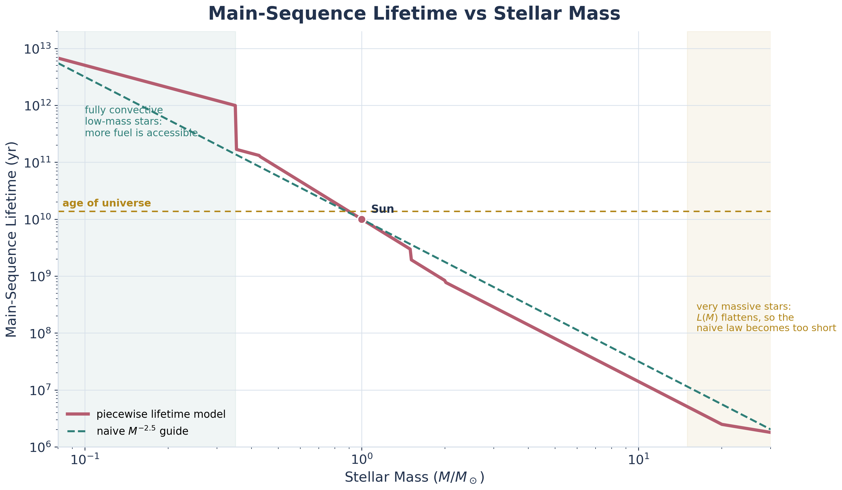
Now the mass-luminosity relation — the crown jewel of Module 2 — pays off. For main-sequence stars $L \propto M^{3.5}$ . Substituting into the nuclear timescale:

One of the most important scaling relations in all of astrophysics.

Notice the move you just made — you will make it again all module. Take a relation you already trust ( $\tau_\text{nuc} \sim \varepsilon f_M Mc^2/L$ ), substitute a known scaling ( $L \propto M^{3.5}$ ), and read off how the quantity must depend on mass — no differential equation solved, just its structure read. The price of admission is naming what you leaned on: that the $L$ – $M$ relation holds and that $\varepsilon$ and $f_M$ stay roughly constant from star to star. That habit — read the equation, extract the scaling, name the assumption — is the through-line of Module 3. In the next reading you will run it on the equation of stellar structure itself, this time by approximating a derivative.

Generated white-background log-log plot comparing accessible fuel reservoir and luminosity burn rate as functions of stellar mass, with labeled representative stars at 0.2, 1, and 10 solar masses. — Figure 3The accessible fuel reservoir increases with stellar mass, but the luminosity increases much faster. That is the visual reason massive stars die young.ASTR 201 (generated)

Star Mass ( $M/M_\odot$ )	Lifetime ( $\tau_\text{nuc}$ )	Comparison
$0.1$	$\sim 3 \times 10^{12}~\text{yr}$	Simple scaling only; still far beyond the age of the universe
$0.5$	$\sim 56~\text{Gyr}$	Longer than the universe’s age — still on the MS
$1.0$	$\sim 10~\text{Gyr}$	Sun: halfway through
$2.0$	$\sim 1.8~\text{Gyr}$	Short enough to see evolution in clusters
$10$	$\sim 32~\text{Myr}$	Geologically brief

The pattern is dramatic. A $10\,M_\odot$ star has 10 times the fuel but burns it $10^{3.5} \approx 3{,}000$ times faster, so its lifetime is $\sim 1/300$ of the Sun’s. A $0.1\,M_\odot$ red dwarf has $1/10$ the fuel but burns it $\sim 3{,}000$ times slower — it will outlive the current universe by a factor of a couple hundred. Two caveats: at low mass the luminosity scaling changes and fully convective stars access more of their hydrogen, so the lowest-mass stars live even longer than $M^{-2.5}$ suggests; at high mass the $L$ - $M$ relation bends, so extrapolating to $50$ – $100\,M_\odot$ predicts lifetimes that are too short. The scaling still gets the right qualitative story and order of magnitude across the broad middle of the main sequence.

Generated white-background log-log plot of main-sequence lifetime versus stellar mass showing a solid piecewise lifetime model, a dashed naive M to the minus 2.5 guide, a Sun marker, an age-of-the-universe line, and shaded caveat regions for fully convective low-mass stars and very massive stars. — Figure 4The naive tau proportional to M^-2.5 guide captures the broad trend, but real low-mass stars live even longer because they access more of their fuel, while very massive-star lifetimes exceed a blind high-mass extrapolation.ASTR 201 (generated)

Worked Example 4Why M Dwarfs Live So Long

Problem

Take an idealized fully convective M dwarf with $M/M_\odot = 0.2$ , $L/L_\odot \approx (0.2)^{3.5} \approx 0.0036$ , and (because full convection mixes more fuel) $f_M/f_{M,\odot} \approx 10$ . Estimate its main-sequence lifetime.

StepSolar-normalized nuclear lifetime

$\frac{\tau_\text{nuc}}{\tau_{\text{nuc},\odot}} \approx \left(\frac{f_M}{f_{M,\odot}}\right)\left(\frac{M}{M_\odot}\right)\left(\frac{L}{L_\odot}\right)^{-1} \approx 10 \times 0.2 \times (0.0036)^{-1} \approx 560$

Dimensional check

Every factor is a dimensionless solar ratio; the product is dimensionless, and units enter only via the Sun’s $\sim 10~\text{Gyr}$ ✓.

Result

$\tau_\text{nuc} \approx 560 \times 10~\text{Gyr} \approx 5.6 \times 10^{12}~\text{yr}$ — about 5.6 trillion years, far longer than the universe’s age. This is why the faintest red dwarfs are the Galaxy’s long-term survivors. (Not an exact prediction — it combines the simple luminosity scaling with a convection-boosted fuel fraction — but the conclusion is robust.)

Misconception check — more fuel means a longer life

A student says, “A more massive star must live longer — look how much more hydrogen it has to burn.” Where does this reasoning break?

Multiple choice

A more massive star should live longer because it contains more hydrogen fuel.

TrueFalse

Numeric answer

A star in a young cluster is spectral type B2 ( $M \approx 10\,M_\odot$ ) and still on the main sequence. Estimate the nuclear timescale of a $10\,M_\odot$ star — the upper bound on the cluster’s age.

Your answer

The Hierarchy of Timescales

Part 5: The Hierarchy of Timescales

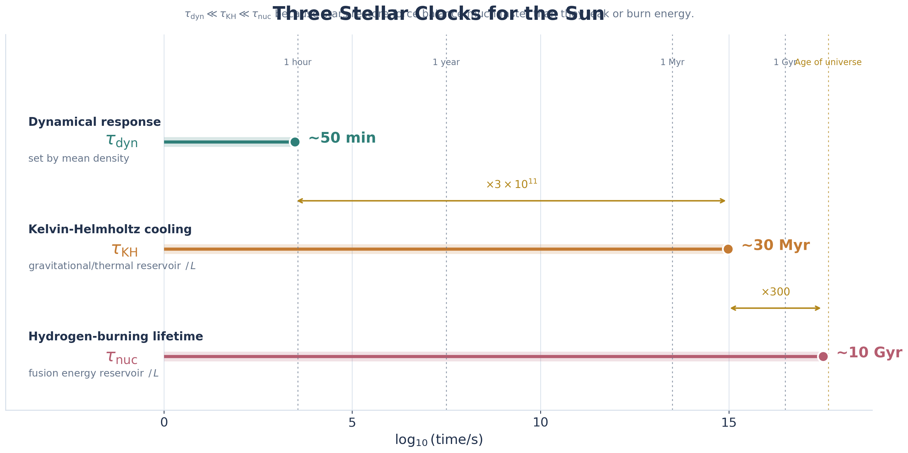
White-background comparison plot for the Sun's three stellar timescales with labeled bars for dynamical response, Kelvin-Helmholtz cooling, and nuclear lifetime, plus reference markers for hour, year, Myr, Gyr, and the age of the universe. — Figure 5The three stellar clocks are separated by enormous factors. The Kelvin-Helmholtz and nuclear timescales both follow the 'reservoir divided by luminosity' logic, while the dynamical clock is set by mean density.ASTR 201 (generated)

For the Sun, the three timescales span an enormous range — each answering a different physical question: mechanical response, thermal depletion, fuel exhaustion.

Timescale	Symbol	Value (Sun)	Physical Process
Dynamical	$\tau_\text{dyn}$	$\sim 50~\text{min}$	Free-fall / pressure response
Thermal (KH)	$\tau_\text{KH}$	$\sim 30~\text{Myr}$	Quasi-static contraction on the binding-energy reservoir
Nuclear	$\tau_\text{nuc}$	$\sim 10~\text{Gyr}$	Hydrogen fusion

The hierarchy $\tau_\text{dyn} \ll \tau_\text{KH} \ll \tau_\text{nuc}$ has profound consequences:

The star is in dynamical equilibrium. Because $\tau_\text{dyn}$ is so short (minutes), any departure from pressure-gravity balance is corrected almost instantly — which is why stars are (nearly) in hydrostatic equilibrium at all times (formalized in the next reading).
Thermal adjustments are slow but finite. If the nuclear source were suddenly switched off, the star wouldn’t collapse instantly — it would slowly contract and radiate its stored thermal energy over $\tau_\text{KH} \sim 30~\text{Myr}$ .
Nuclear burning sets the true lifetime. Because $\tau_\text{nuc} \gg \tau_\text{KH}$ , the star has ample time to establish thermal equilibrium while burning fuel, shining steadily for billions of years.

Why This Hierarchy Matters

The separation of timescales is why stars exist as stable, luminous objects. If $\tau_\text{dyn}$ were comparable to $\tau_\text{nuc}$ , stars would pulsate wildly; if $\tau_\text{KH}$ were comparable to $\tau_\text{nuc}$ , stars couldn’t establish thermal equilibrium before their fuel ran out. The enormous separation $\tau_\text{dyn} \ll \tau_\text{KH} \ll \tau_\text{nuc}$ lets us treat stars as quasi-static objects evolving slowly through equilibrium states — the simplification that makes stellar physics tractable.

Observable

The main-sequence turnoff of a star cluster

In a coeval cluster, the most luminous (most massive) star still on the main sequence — the turnoff point — is directly read off the cluster’s HR diagram.

Model

Nuclear lifetime from the mass-luminosity relation

$\tau_\text{nuc} \propto M^{-2.5}$ : the turnoff mass maps to a main-sequence lifetime.

Inference

The cluster's age

Cluster age $\approx \tau_\text{nuc}$ of the turnoff star. Blue (massive) turnoffs mean young clusters; red (low-mass) turnoffs mean old ones.

Quick check

From Module 2 you read a young cluster’s HR diagram and find its main-sequence turnoff at $M \approx 5\,M_\odot$ . Which of the three timescales turns that single observation into the cluster’s age — and why are the other two the wrong tool here?

Multiple choice

Rank fastest to slowest: (a) the Sun responding to a sudden pressure disturbance, (b) the Sun exhausting its hydrogen fuel, (c) a hypothetical Sun (no nuclear source) radiating away its stored gravitational energy.

a < c < b

(dynamical, then Kelvin–Helmholtz, then nuclear)

a < b < c

c < a < b

b < c < a

Reference and Synthesis

Reference Tables

The Three Stellar Timescales

Timescale	Formula	Physical Meaning	Sun Value
Dynamical $\tau_\text{dyn}$	$\sim 1/\sqrt{G\bar{\rho}}$	Free-fall time; how fast gravity rearranges matter	$\sim 50~\text{min}$
Thermal $\tau_\text{KH}$	$\sim GM^2/(RL)$	Time to radiate the binding-energy reservoir	$\sim 30~\text{Myr}$
Nuclear $\tau_\text{nuc}$	$\sim \varepsilon f_M Mc^2/L$	Time to exhaust nuclear fuel	$\sim 10~\text{Gyr}$

Symbol Legend

Symbol	Meaning	CGS Units
$G$	Newton’s gravitational constant	$6.674 \times 10^{-8}~\text{cm}^3\text{g}^{-1}\text{s}^{-2}$
$\bar{\rho}$	Mean density	$\text{g cm}^{-3}$
$M$	Stellar mass	g (or $M_\odot = 2.0 \times 10^{33}~\text{g}$ )
$R$	Stellar radius	cm (or $R_\odot = 7.0 \times 10^{10}~\text{cm}$ )
$L$	Luminosity	erg/s (or $L_\odot = 3.8 \times 10^{33}~\text{erg/s}$ )
$c$	Speed of light	$3.0 \times 10^{10}~\text{cm/s}$
$\varepsilon$	Nuclear conversion efficiency	dimensionless ( $\approx 0.007$ for H→He)
$f_M$	Accessible fuel fraction ( $f_M M$ actually burns)	dimensionless ( $\approx 0.10$ for a Sun-like star)

Summary: Stars Are Clocks

Three timescales govern stellar physics — dynamical ( $\sim$ minutes), thermal ( $\sim$ Myr), and nuclear ( $\sim$ Gyr) — and their hierarchy $\tau_\text{dyn} \ll \tau_\text{KH} \ll \tau_\text{nuc}$ makes stars stable, quasi-static objects.
The Kelvin-Helmholtz controversy showed that observations (geological ages) can demand new physics (nuclear energy). Kelvin’s calculation was correct; his assumptions were incomplete.
Nuclear lifetime scales as $\tau_\text{nuc} \propto M^{-2.5}$ — massive stars burn far faster than they gain extra fuel. A $10\,M_\odot$ star lives $\sim 30~\text{Myr}$ ; a $0.1\,M_\odot$ star outlasts the universe.
The main-sequence turnoff gives cluster ages: the most massive star still on the MS sets the clock.

Where we stand · Reading 1 of 5

The through-line of Module 3: what holds a star up, and what makes it shine?

✓ Settled. Three clocks govern a star, and their separation — $\tau_\text{dyn} \ll \tau_\text{KH} \ll \tau_\text{nuc}$ — is what lets us model it as a static, balanced structure. The longest, $\tau_\text{nuc} \propto M^{-2.5}$ , sets the lifetime.

? Still open. What actually holds the star up — and powers it for $\sim 10~\text{Gyr}$ ? Gravity alone would collapse the Sun in $\sim 50$ minutes, yet it has shone steadily for $4.6~\text{Gyr}$ . Something balances gravity, and something keeps replenishing what it radiates.

→ Next. What force balances gravity? Reading 2 — hydrostatic equilibrium.

Quick retrieval: a cluster still showing blue main-sequence turnoff stars — is it young or old?

Looking Ahead

You now know stars live for $\tau_\text{nuc} \propto M^{-2.5}$ — but why do they last this long? What holds them up against gravity, and what generates the energy that maintains the balance? In Reading 2 the answer is hydrostatic equilibrium — the precise balance between gravity’s inward pull and pressure’s outward push. And in Reading 3, the energy source maintaining that balance turns out to demand all four fundamental forces of nature, including quantum mechanics. Keep one number in your pocket as you go: $\tau_\text{nuc} \propto M^{-2.5}$ . It means every star is born onto a clock that runs out — fast for the massive, almost never for the faint — and what happens when it runs out is where the second half of this module is headed: how stars age, swell, and die.

Glossary

Dynamical timescale: The characteristic time for gravity to rearrange a star if pressure support failed: $\tau_\text{dyn} \sim 1/\sqrt{G\bar{\rho}}$ — about 50 minutes for the Sun. The shortest of the three stellar clocks; it sets how fast a star restores hydrostatic equilibrium after a perturbation.
Kelvin-Helmholtz timescale: The time a star could shine on gravitational contraction alone: $\tau_\text{KH} \sim GM^2/(RL)$ — about 30 Myr for the Sun. It is a quasi-static contraction time, not a free fall; nuclear fusion makes the real lifetime hundreds of times longer.
Main-sequence turnoff: The point on a star cluster’s HR diagram where the most massive stars are just leaving the main sequence. Because nuclear lifetime falls steeply with mass, the turnoff mass is a clock: a high (blue) turnoff means a young cluster, a low (red) turnoff an old one.
Nuclear timescale: The time core hydrogen fusion can sustain a star’s luminosity: $\tau_\text{nuc} \sim \varepsilon f_M M c^2 / L$ — about 10 Gyr for the Sun. It is the longest of the three clocks and sets a star’s true main-sequence lifetime.