title: “Chapter 7: NumPy - The Foundation of Scientific Computing” subtitle: “COMP 536 | Scientific Computing Core” author: “Anna Rosen” draft: false execute: echo: true format: html: toc: true —
Learning Objectives
By the end of this chapter, you will be able to:
Prerequisites Check
Before starting this chapter, verify you can:
Self-Assessment Diagnostic
Test your readiness by predicting these outputs WITHOUT running the code:
# Question 1: What does this produce?result = [x**2for x inrange(5) if x %2==0]# Your answer: _______# Question 2: What's the final value of total?total =sum([len(str(x)) for x in [10, 100, 1000]])# Your answer: _______# Question 3: What error (if any) occurs here?import mathvalues = [1, 4, 9]# roots = math.sqrt(values) # Uncomment to test# Your answer: _______# Question 4: Can you understand this nested structure?matrix = [[1, 2], [3, 4]]flattened = [item for row in matrix for item in row]# Your answer: _______
TipSelf-Assessment Answers
[0, 4, 16] - squares of even numbers from 0-4
9 - lengths are 2, 3, 4, sum = 9
TypeError - math.sqrt() doesn’t accept lists, only single values
[1, 2, 3, 4] - flattens the 2D list into 1D
If you got all four correct, you’re ready for NumPy! If not, review the indicated chapters.
Chapter Overview
You’ve been using Python lists to store collections of numbers, and the math module to perform calculations. But what happens when you need to analyze a million stellar spectra, each with thousands of wavelength points? Or when you need to perform the same calculation on every pixel in a telescope image? Try using a list comprehension on a million-element list, and you’ll be waiting a while. This is where NumPy transforms Python from a general-purpose language into a powerhouse for scientific computing, providing the speed and tools necessary for research-grade computational science.
NumPy, short for Numerical Python, is the foundation upon which the entire scientific Python ecosystem is built. Every plot you’ll make with Matplotlib, every optimization you’ll run with SciPy, every dataframe you’ll analyze with Pandas – they all build on NumPy arrays. But NumPy isn’t just about speed; it’s about expressing mathematical operations naturally. Instead of writing loops to add corresponding elements of two lists, you simply write a + b. Instead of nested loops for matrix multiplication, you write a @ b. This isn’t just convenience – it’s a fundamental shift in how you think about numerical computation, from operating on individual elements to operating on entire arrays at once.
This chapter introduces you to NumPy’s ndarray (n-dimensional array), the object that makes scientific Python possible. You’ll discover why NumPy arrays are often much faster than Python lists for numerical operations, and how vectorization eliminates the need for most explicit loops. You’ll master broadcasting, NumPy’s powerful mechanism for operating on arrays of different shapes, which enables elegant solutions to complex problems. Most importantly, you’ll learn to think in arrays – a skill that transforms you from someone who writes code that processes data to someone who writes code that expresses mathematical ideas directly. The examples lean astro‑flavored, but the patterns apply just as well to climate, biology, imaging, and signal processing.
This chapter introduces NumPy’s core concepts, but NumPy is vast! The official documentation at https://numpy.org/doc/stable/ is your indispensable companion. Throughout your career, you’ll constantly reference it for:
Complete function signatures and parameters
Advanced broadcasting examples
Performance optimization tips
Specialized submodules (random, fft, linalg)
Practice using the documentation NOW: After each new function you learn, look it up in the official docs. Read the parameters, check the examples, and explore related functions. The ability to efficiently navigate documentation is as important as coding itself. Bookmark the NumPy documentation – you’ll use it daily in research!
Pro tip: Use the NumPy documentation’s search function to quickly find what you need. Type partial function names or concepts, and it will suggest relevant pages. The “See Also” sections are goldmines for discovering related functionality.
7.1 From Lists to Arrays: Why NumPy?
NumPy A fundamental package for scientific computing in Python, providing support for large, multi-dimensional arrays and matrices.
ndarray NumPy’s n-dimensional array object, the core data structure for numerical computation.
Contiguous Memory Data stored in adjacent memory locations, enabling fast access and cache efficiency.
Let’s start with a problem you already know how to solve, then see how NumPy transforms it. Imagine you’re analyzing brightness measurements from a variable star:
import timeimport math# Python list approach (what you know from Chapter 4)magnitudes_list = [12.3, 12.5, 12.4, 12.7, 12.6] *20000# 100,000 measurementsfluxes = []start = time.perf_counter()for mag in magnitudes_list: flux =10**(-mag/2.5) # Convert magnitude to relative flux fluxes.append(flux)list_time = time.perf_counter() - startprint(f"List approach: {list_time*1000:.2f} ms")print(f"First 5 fluxes: {fluxes[:5]}")
List approach: 10.43 ms
First 5 fluxes: [1.2022644346174132e-05, 1e-05, 1.0964781961431852e-05, 8.31763771102671e-06, 9.120108393559096e-06]
Now let’s see the NumPy approach:
import timeimport numpy as np # Standard abbreviation used universally# NumPy array approach (what you're learning)magnitudes = np.array([12.3, 12.5, 12.4, 12.7, 12.6] *20000)start = time.perf_counter()fluxes_np =10**(-magnitudes/2.5) # Operates on entire array at once!numpy_time = time.perf_counter() - startprint(f"NumPy approach: {numpy_time*1000:.2f} ms")print(f"Speedup: {list_time/numpy_time:.1f}x faster")print(f"First 5 fluxes: {fluxes_np[:5]}")
NumPy approach: 5.07 ms
Speedup: 2.1x faster
First 5 fluxes: [1.20226443e-05 1.00000000e-05 1.09647820e-05 8.31763771e-06
 9.12010839e-06]
The NumPy version is not only faster but also cleaner – no explicit loop needed! This is called vectorization, and it’s the key to NumPy’s power.
NumPy vs. the math Module: Arrays vs. Scalars
You’ve been using the math module for operations like math.sin(), math.sqrt(), and math.log(). NumPy covers most of the same operations while adding array support, which is why it becomes the default tool in scientific computing:
# Math module - works on single values onlyimport mathx =2.0math_result = math.sin(x)print(f"math.sin({x}) = {math_result}")# Try with a list - this fails!# values = [0, 1, 2, 3]# math.sin(values) # TypeError!# NumPy - works on single values AND arraysx =2.0numpy_scalar_result = np.sin(x)print(f"np.sin({x}) = {numpy_scalar_result}")# NumPy shines with arraysvalues = np.array([0, 1, 2, 3])numpy_array_result = np.sin(values)print(f"np.sin({values}) = {numpy_array_result}")# NumPy has everything math has (and more)print(f"\nComparison for x = {x}:")print(f" math.sqrt({x}) = {math.sqrt(x):.6f}")print(f" np.sqrt({x}) = {np.sqrt(x):.6f}")print(f" math.exp({x}) = {math.exp(x):.6f}")print(f" np.exp({x}) = {np.exp(x):.6f}")print(f" math.log10({x}) = {math.log10(x):.6f}")print(f" np.log10({x}) = {np.log10(x):.6f}")
Key insight: For arrays, prefer NumPy. For scalar-only work, math is perfectly fine. A few specialized functions live in math or scipy.special, so use the tool that matches the problem.
NoteQuick Check
You need square roots for a single number and for a whole array. Which module would you use for each, and why?
Note🎯 The More You Know: NumPy Powers Gravitational Wave Detection
In the mid-2010s, the Laser Interferometer Gravitational-Wave Observatory (LIGO) detected gravitational waves for the first time, opening a new window on the universe. This discovery depended on sophisticated data analysis pipelines, including PyCBC, which relies heavily on NumPy.
Astro example — the same signal‑processing workflow appears in seismology, acoustics, and medical imaging.
LIGO’s detectors produce high-rate, noisy data streams. Detecting a gravitational wave requires comparing those streams against large banks of theoretical waveform templates using matched filtering — a computationally intensive process that would be impossible without efficient numerical libraries.
The PyCBC pipeline is built on NumPy arrays and operations. The power of NumPy’s vectorized operations, which call optimized compiled routines (often BLAS/LAPACK; FFT via optimized routines), enables the analysis of gravitational wave data at practical timescales. Here’s how NumPy transforms the core matched filtering operation:
# Traditional loop-based approachdef matched_filter_slow(data, template): result =0for i inrange(len(data)): result += data[i] * template[i]return result# NumPy vectorized approachdef matched_filter_fast(data, template):return np.dot(data, template) # Or simply: data @ template
The vectorized NumPy version is dramatically faster, enabling searches through large template banks. NumPy’s FFT implementation accelerates the frequency-domain operations that are central to the analysis.
Today, gravitational-wave detections are processed through analysis pipelines built on NumPy arrays. The library you’re learning provides the computational foundation for this new kind of astronomy.
7.2 Creating Arrays: Your Scientific Data Containers
dtype Data type of array elements, controlling memory usage and precision.
NumPy provides many ways to create arrays, each suited for different scientific tasks:
# From Python lists (most common starting point)measurements = [23.5, 24.1, 23.8, 24.3]arr = np.array(measurements)print(f"From list: {arr}, dtype: {arr.dtype}")# Specify data type for memory efficiencycounts = np.array([1000, 2000, 1500], dtype=np.int32)print(f"Integer array: {counts}, dtype: {counts.dtype}")# 2D array (matrix) - like an imageimage_data = np.array([[10, 20, 30], [40, 50, 60], [70, 80, 90]])print(f"2D array shape: {image_data.shape}")print(f"2D array:\n{image_data}")
Essential Array Creation Functions for Science
CGS Units Centimeter-Gram-Second system, traditionally used in astronomy and astrophysics.
These functions are workhorses in scientific computing:
Unit clarity matters: even without a units library, include units in variable names (e.g., wavelengths_nm, mass_g) and stay consistent within a workflow.
# linspace: Evenly spaced values (inclusive endpoints)# Perfect for wavelength grids, time serieswavelengths_nm = np.linspace(400, 700, 11) # 11 points from 400 to 700 nmprint(f"Wavelengths (nm): {wavelengths_nm}")# Convert to CGS (cm) - standard in stellar atmosphere modelswavelengths_cm = wavelengths_nm *1e-7print(f"Wavelengths (cm): {wavelengths_cm}")# logspace: Logarithmically spaced values# Essential for frequency grids, stellar massesmasses_solar = np.logspace(-1, 2, 4) # 0.1 to 100 solar massesmasses_g = masses_solar *1.989e33# Convert to grams (CGS)print("Stellar masses (g):", ", ".join(f"{x:.2e}"for x in masses_g))
# arange: Like Python's range but returns arraytimes_s = np.arange(0, 10, 0.1) # 0 to 9.9 in 0.1s stepsprint(f"Time points: {len(times_s)} samples from {times_s[0]} to {times_s[-1]}")# zeros and ones: Initialize arraysdark_frame = np.zeros((100, 100)) # 100x100 CCD dark frameflat_field = np.ones((100, 100)) # Flat field (perfect response)print(f"Dark frame shape: {dark_frame.shape}, sum: {dark_frame.sum()}")print(f"Flat field shape: {flat_field.shape}, sum: {flat_field.sum()}")# full: Create array filled with specific valuebias_level = np.full((100, 100), 500) # CCD bias levelprint(f"Bias array: all values = {bias_level[0, 0]}")# eye: Identity matrixidentity = np.eye(3)print(f"Identity matrix:\n{identity}")
Tip💡 Computational Thinking Box: Row-Major vs Column-Major
PATTERN: Memory Layout Matters for Performance
NumPy stores arrays in row-major order (C-style) by default, meaning elements in the same row are adjacent in memory. This affects performance dramatically:
# Row-major (NumPy default) - fast row operationsimage = np.zeros((1000, 1000))# Accessing image[0, :] is fast (contiguous memory)# Accessing image[:, 0] is slower (strided memory)# For column operations, consider Fortran orderimage_fortran = np.zeros((1000, 1000), order='F')# Now image_fortran[:, 0] is fast
Why this matters:
Processing images row-by-row? Use default (C-order)
Processing spectra in columns? Consider Fortran order
Real impact: The wrong memory order can make your code noticeably slower for large arrays!
Note🔍 Check Your Understanding
What’s the memory difference between np.zeros(1000), np.ones(1000), and np.empty(1000)? When would you use each?
TipAnswer
All three allocate the same amount of memory (8000 bytes for float64), but:
np.zeros(): Allocates AND sets all values to 0 (slower, safe)
np.ones(): Allocates AND sets all values to 1 (slower, safe)
np.empty(): Only allocates, doesn’t initialize (fastest, dangerous)
Use cases:
zeros()/ones(): When you need initialized values for accumulation or defaults
empty(): ONLY when you’ll immediately overwrite ALL values, like filling with calculated results
Example where empty() is appropriate:
result = np.empty(1000)for i inrange(1000): result[i] = expensive_calculation(i) # Overwrites immediately
Saving and Loading Arrays (Connection to Chapter 6)
Remember the file I/O concepts from Chapter 6? NumPy extends them for efficient array storage:
import os # For cleanuprng = np.random.default_rng(42)# Save astronomical data in binary formatflux_data = rng.normal(1000, 50, size=1000)np.save('observations.npy', flux_data) # Binary format, fast# Load for analysisloaded_data = np.load('observations.npy')print(f"Loaded {len(loaded_data)} measurements")# For text format (human-readable but slower)np.savetxt('observations.txt', flux_data[:10], fmt='%.2f')text_data = np.loadtxt('observations.txt')print(f"Text file sample: {text_data[:3]}")# Clean up filesos.remove('observations.npy')os.remove('observations.txt')
7.3 Random Numbers for Monte Carlo Simulations
Monte Carlo A computational technique using random sampling to solve problems that might be deterministic in principle.
Scientific computing often requires random data for Monte Carlo simulations, noise modeling, and statistical testing. NumPy’s random module provides a comprehensive suite of distributions essential for computational astrophysics:
NoteNote on Reproducibility
Random number generation can produce slightly different values across NumPy versions and hardware architectures, even with the same seed. The statistical properties remain consistent, but exact values may vary. For reproducible workflows, use the np.random.Generator interface (default_rng) and record both your NumPy version and the bit generator (rng.bit_generator).
Legacy np.random.* functions still exist, but they rely on global state. In new scientific code, prefer a local generator created with np.random.default_rng(...).
Common Distributions
The three distributions you’ll use most frequently are uniform, normal (Gaussian), and Poisson. Master these first before moving to specialized distributions.
Uniform Distribution
Use for random positions, phases, and any quantity that’s equally likely across a range:
import numpy as np# Create a local Generator for reproducibility without global staterng = np.random.default_rng(42)# Uniform distribution: random positions, phases# Generate random sky coordinates uniformly on the spheren_stars =1000ra = rng.uniform(0, 360, n_stars) # Right Ascension in degreesu = rng.uniform(-1, 1, n_stars) # Uniform in sin(dec), not in decdec = np.degrees(np.arcsin(u)) # Declination in degreesprint(f"Generated {n_stars} random sky positions")print(f"RA range: [{ra.min():.1f}, {ra.max():.1f}] deg")# Random phases for periodic variablesphases = rng.uniform(0, 2*np.pi, n_stars)print(f"Phase range: [0, 2pi]")# Shorthand for uniform [0, 1)random_fractions = rng.random(5)print(f"Random fractions: {random_fractions}")
Generated 1000 random sky positions
RA range: [0.4, 359.7] deg
Phase range: [0, 2pi]
Random fractions: [0.82922114 0.59409599 0.24485475 0.745675   0.0844809 ]
Uniform sky coverage is a subtle but important point: equal-area sampling on a sphere means uniform in \(\sin(\mathrm{dec})\), not uniform in declination itself. Sampling dec uniformly would over-weight the poles.
Normal (Gaussian) Distribution
Use for measurement errors, thermal noise, and any quantity resulting from many small independent effects:
# Normal (Gaussian) distribution: measurement errors, thermal noise# Simulate CCD readout noiserng = np.random.default_rng(42)mean_counts =1000# electronsread_noise =10# electrons RMSn_pixels =10000pixel_values = rng.normal(mean_counts, read_noise, n_pixels)print(f"Pixel statistics:")print(f" Mean: {pixel_values.mean():.1f} (expected: {mean_counts})")print(f" Std: {pixel_values.std():.1f} (expected: {read_noise})")print(f" SNR: {pixel_values.mean()/pixel_values.std():.1f}")# Shorthand for standard normal (mean=0, std=1)standard_normal = rng.standard_normal(5)print(f"Standard normal samples: {standard_normal}")
Photon counts, particle detections, cosmic ray hits
Advanced Distributions for Astrophysics
These distributions are less common but essential for specific astrophysical applications.
Exponential Distribution
Use for waiting times between events (time to next supernova, time between cosmic ray hits):
# Exponential distribution: time between events, decay processes# Simulate time between supernova detections (days)rng = np.random.default_rng(42)mean_interval =30# daysn_events =100intervals = rng.exponential(mean_interval, n_events)print(f"Supernova intervals: mean = {intervals.mean():.1f} days")
Supernova intervals: mean = 27.0 days
Power-Law Distribution
Use for stellar masses (IMF), galaxy luminosities, and many astrophysical scaling relations:
# Power-law distribution (using Pareto for x_min=1)# Initial Mass Function approximationrng = np.random.default_rng(42)alpha =2.35# Salpeter IMF slope (dN/dM ∝ M^-alpha)n_stars =1000# Generate masses from 0.1 to 100 solar massesa = alpha -1# np.random.pareto(a) has p(x) ∝ x^-(a+1)x = rng.pareto(a, n_stars) +1# Pareto starts at 1masses =0.1* x # Scale to start at 0.1 solar massesmasses = masses[masses <100] # Truncate at 100 solar massesprint(f"Generated {len(masses)} stellar masses with power-law distribution")
Generated 1000 stellar masses with power-law distribution
This is a classic “parameter name mismatch” moment: NumPy’s pareto(a) returns a distribution with \(p(x) \propto x^{-(a+1)}\), while the Salpeter IMF is \(dN/dM \propto M^{-\alpha}\). Matching the exponents means using \(a = \alpha - 1\).
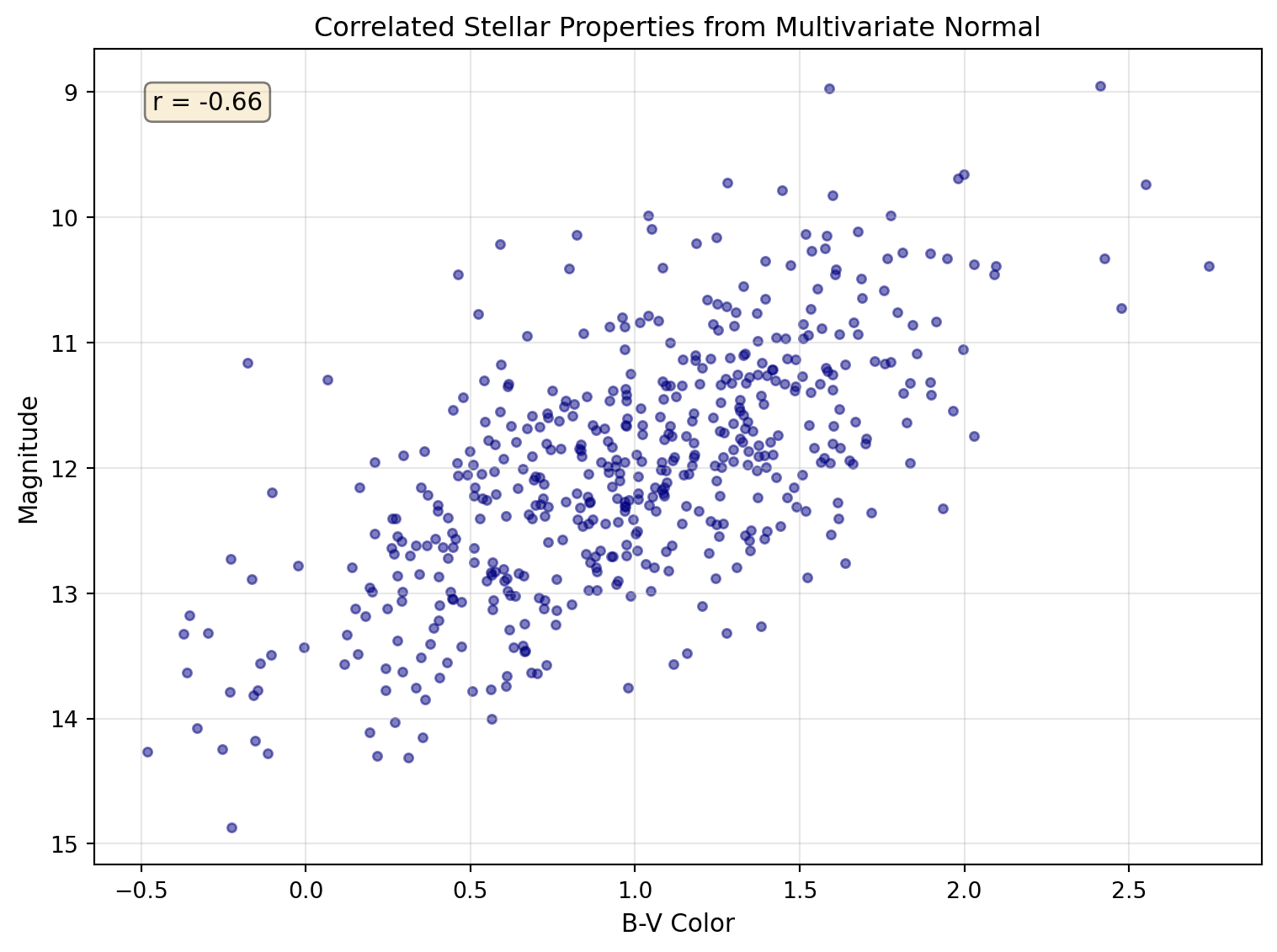
Multivariate Normal Distribution
Use for correlated parameters (color-magnitude relationships, correlated measurement errors):
# Multivariate normal: correlated parameters# Simulate color-magnitude relationshiprng = np.random.default_rng(42)mean = [12, 1.0] # Mean magnitude, mean color (B-V)# Covariance matrix: brighter stars tend to be bluercov = [[1.0, -0.3], # Variance in mag, covariance [-0.3, 0.25]] # Covariance, variance in colorn_stars =500mag_color = rng.multivariate_normal(mean, cov, n_stars)magnitudes = mag_color[:, 0]colors = mag_color[:, 1]correlation = np.corrcoef(magnitudes, colors)[0, 1]print(f"Generated {n_stars} stars with correlated properties")print(f"Correlation coefficient: {correlation:.2f} (expected: ~-0.6)")
Multivariate normal distribution showing correlated stellar properties. The elliptical shape reveals the negative correlation between magnitude and color.
Random Sampling Techniques
Weighted Random Choice
Use for selecting objects from catalogs with known probability distributions:
Important🌟 Why This Matters: Monte Carlo Markov Chain (MCMC) in Cosmology
The random number generation you’re learning powers one of modern cosmology’s most important techniques: MCMC sampling for parameter estimation. When analyzing the cosmic microwave background or galaxy surveys, we need to explore vast parameter spaces to find the best-fit cosmological model.
Astro example — the same Monte Carlo ideas show up in ecology, materials science, and Bayesian machine learning.
MCMC uses random walks through parameter space, with each step drawn from distributions like those above. Missions such as Planck used these methods to place tight constraints on the universe’s age, composition, and expansion history.
Your ability to generate and manipulate random numbers with NumPy is the foundation for these universe-spanning discoveries.
7.4 Array Operations: Vectorization Powers
Vectorization Performing operations on entire arrays at once rather than using explicit loops.
Universal Functions NumPy functions that operate element-wise on arrays, supporting broadcasting and type casting.
The true power of NumPy lies in vectorized operations – performing calculations on entire arrays without writing loops:
NumPy’s universal functions operate element-wise on arrays with optimized C code:
# Trigonometric functions for coordinate transformationsangles_deg = np.array([0, 30, 45, 60, 90])angles_rad = np.deg2rad(angles_deg) # Convert to radianssines = np.sin(angles_rad)cosines = np.cos(angles_rad)print(f"Angles (deg): {angles_deg}")print(f"sin(theta): {sines}")print(f"cos(theta): {cosines}")print(f"sin^2(theta) + cos^2(theta): {sines**2+ cosines**2}") # Should all be 1!
# Exponential and logarithm for magnitude scalesmagnitudes = np.array([0, 1, 2, 5, 10])flux_ratios =10**(-magnitudes/2.5) # Pogson's equationprint(f"\nMagnitudes: {magnitudes}")print(f"Flux ratios: {flux_ratios}")# Verify: magnitude difference = -2.5 * log10(flux ratio)recovered_mags =-2.5* np.log10(flux_ratios)print(f"Recovered magnitudes: {recovered_mags}")# Floating point comparison - use allclose for safetyprint(f"Magnitudes match: {np.allclose(magnitudes, recovered_mags)}")
Array Methods: Built-in Analysis
Arrays come with methods for common statistical operations:
# Create sample data: Gaussian with outliersrng = np.random.default_rng(42)data = rng.normal(100, 15, 1000) # Normal dist: mean=100, std=15data[::100] =200# Add outliers every 100th point# Statistical methodsprint(f"Mean: {data.mean():.2f}")print(f"Median: {np.median(data):.2f}") # More robust to outliersprint(f"Std dev (population): {data.std():.2f}")print(f"Std dev (sample, ddof=1): {data.std(ddof=1):.2f}")print(f"Min: {data.min():.2f}, Max: {data.max():.2f}")# Find outliersoutliers = data >150n_outliers = outliers.sum() # True counts as 1print(f"Number of outliers (>150): {n_outliers}")# Clean data by filteringclean_data = data[~outliers] # ~ means NOTprint(f"Clean mean: {clean_data.mean():.2f}")print(f"Clean std: {clean_data.std():.2f}")# Additional useful statisticsprint(f"\nPercentiles:")print(f" 25th: {np.percentile(data, 25):.2f}")print(f" 75th: {np.percentile(data, 75):.2f}")print(f" 95th: {np.percentile(data, 95):.2f}")
Warning⚠️ Common Bug Alert: Integer Division Trap
# DANGER: Integer arrays can cause unexpected results!counts = np.array([100, 200, 300]) # Default type is intnormalized = counts / counts.max()print(f"Normalized (float result): {normalized}")# But watch out for integer division with //integer_div = counts //2# Floor divisionprint(f"Integer division by 2: {integer_div}")# Mixed operations preserve precisioncounts_int = np.array([100, 200, 300], dtype=int)scale =2.5# floatscaled = counts_int / scale # Result is float!print(f"Int array / float = {scaled}")# Best practice: Use float arrays for scientific calculationscounts_safe = np.array([100, 200, 300], dtype=float)print(f"Safe float array: {counts_safe / counts_safe.max()}")
Always use float arrays for scientific calculations unless you specifically need integer arithmetic!
Tip💡 Computational Thinking Box: Algorithmic Complexity and Big-O
PATTERN: Understanding Algorithmic Scaling
Different approaches to the same problem can have vastly different performance:
# O(n) - Linear time with Python loopdef sum_squares_loop(arr): total =0for x in arr: total += x**2return total# O(n) - Linear time with NumPy (but ~100x faster!)def sum_squares_numpy(arr):return (arr**2).sum()# O(n^3) - Cubic time for naive matrix multiplicationdef matrix_multiply_loops(A, B): n =len(A) C = [[0]*n for _ inrange(n)]for i inrange(n):for j inrange(n):for k inrange(n): C[i][j] += A[i][k] * B[k][j]return C# O(n^3) - Optimized with NumPy using BLASdef matrix_multiply_numpy(A, B):return A @ B
Real impact (varies by hardware): For a \(1000 \times 1000\) matrix:
Nested loops: seconds
NumPy with optimized BLAS: milliseconds
That’s the difference between waiting and real-time processing!
Note: While algorithms like Strassen’s achieve \(O(n^{2.807})\) complexity theoretically, NumPy uses highly optimized BLAS libraries that, despite being \(O(n^3)\), are typically faster in practice due to cache optimization, vectorization, and parallel processing.
7.5 Indexing and Slicing: Data Selection Mastery
Boolean Masking Using boolean arrays to select elements that meet certain conditions.
NumPy’s indexing extends Python’s list indexing with powerful new capabilities:
# where: conditional operations and finding indicesdata = np.array([1, 5, 3, 8, 2, 9, 4])high_indices = np.where(data >5)[0] # Returns tuple, we want first elementprint(f"Indices where data > 5: {high_indices}")print(f"Values at those indices: {data[high_indices]}")# Conditional replacementclipped = np.where(data >5, 5, data) # Clip values above 5print(f"Clipped data: {clipped}")# clip: cleaner way to bound valuesclipped_better = np.clip(data, 2, 8) # Clip to range [2, 8]print(f"Clipped with np.clip: {clipped_better}")
# unique: find unique values in catalogsstar_types = np.array(['G', 'K', 'M', 'G', 'K', 'G', 'M', 'M', 'K'])unique_types, counts = np.unique(star_types, return_counts=True)print(f"Unique star types: {unique_types}")print(f"Counts: {counts}")# histogram: bin data for analysisrng = np.random.default_rng(42)magnitudes = rng.normal(12, 2, 1000)hist, bins = np.histogram(magnitudes, bins=20)print(f"Histogram has {len(hist)} bins")print(f"Bin edges from {bins[0]:.1f} to {bins[-1]:.1f}")print(f"Peak bin has {hist.max()} stars")# Check for NaN and Inf valuestest_array = np.array([1.0, np.nan, 3.0, np.inf, 5.0])print(f"\nNaN check: {np.isnan(test_array)}")print(f"Inf check: {np.isinf(test_array)}")print(f"Finite check: {np.isfinite(test_array)}")
Handling Missing Data: NaN Patterns
Real scientific data is messy. Telescope observations have bad pixels, surveys have non-detections, and data pipelines occasionally produce invalid values. NumPy’s np.nan (Not a Number) represents these missing or invalid values, but working with NaN requires special care.
Warning⚠️ NaN Propagation Warning
NaN values propagate through calculations silently—one NaN can contaminate an entire analysis!
import numpy as np# NaN propagates through operationsdata = np.array([1.0, 2.0, np.nan, 4.0, 5.0])print(f"Sum with NaN: {data.sum()}") # Returns nan!print(f"Mean with NaN: {data.mean()}") # Returns nan!
Sum with NaN: nan
Mean with NaN: nan
Always check for and handle NaN values before analysis.
Detecting NaN Values
# Create data with missing values (common in astronomical catalogs)magnitudes = np.array([12.5, np.nan, 14.2, np.nan, 11.8, 15.3])print(f"Data: {magnitudes}")print(f"Is NaN: {np.isnan(magnitudes)}")print(f"Number of NaN values: {np.isnan(magnitudes).sum()}")print(f"Any NaN present: {np.any(np.isnan(magnitudes))}")
Data: [12.5  nan 14.2  nan 11.8 15.3]
Is NaN: [False  True False  True False False]
Number of NaN values: 2
Any NaN present: True
Standard functions (corrupted by NaN):
  np.mean(): nan
  np.std(): nan
  np.sum(): nan

NaN-safe functions (ignore NaN):
  np.nanmean(): 13.45
  np.nanstd(): 1.38
  np.nansum(): 53.80
  np.nanmin(): 11.80
  np.nanmax(): 15.30
  np.nanmedian(): 13.35
Strategy 3: Replace NaN Values
Sometimes you want to fill NaN with a specific value:
# Replace NaN with specific valuesmagnitudes = np.array([12.5, np.nan, 14.2, np.nan, 11.8, 15.3])# Replace with a constant (e.g., detection limit)filled_constant = np.where(np.isnan(magnitudes), 99.99, magnitudes)print(f"Filled with 99.99: {filled_constant}")# Replace with the mean of valid valuesmean_val = np.nanmean(magnitudes)filled_mean = np.where(np.isnan(magnitudes), mean_val, magnitudes)print(f"Filled with mean ({mean_val:.2f}): {filled_mean}")# Using np.nan_to_num for NaN and Infdata_with_inf = np.array([1.0, np.nan, np.inf, -np.inf, 5.0])cleaned = np.nan_to_num(data_with_inf, nan=0.0, posinf=1e10, neginf=-1e10)print(f"nan_to_num result: {cleaned}")
Filled with 99.99: [12.5  99.99 14.2  99.99 11.8  15.3 ]
Filled with mean (13.45): [12.5  13.45 14.2  13.45 11.8  15.3 ]
nan_to_num result: [ 1.e+00  0.e+00  1.e+10 -1.e+10  5.e+00]
Strategy 4: Interpolate Over NaN
For time series data, interpolate missing values:
# Linear interpolation over NaN valuestime = np.array([0, 1, 2, 3, 4, 5])flux = np.array([1.0, 1.2, np.nan, np.nan, 1.1, 0.9])# Find valid and invalid indicesvalid_mask =~np.isnan(flux)valid_time = time[valid_mask]valid_flux = flux[valid_mask]# Interpolate at all time pointsinterpolated_flux = np.interp(time, valid_time, valid_flux)print(f"Original: {flux}")print(f"Interpolated: {interpolated_flux}")
Original: [1.  1.2 nan nan 1.1 0.9]
Interpolated: [1.         1.2        1.16666667 1.13333333 1.1        0.9       ]
Tip💡 NaN Handling Best Practices
Check early: Always check for NaN at the start of analysis
Document the source: Know why NaN values exist (non-detections vs bad data)
Choose strategy wisely:
Filter for statistics (mean, std)
Replace for algorithms that can’t handle NaN
Interpolate for time series with small gaps
Use NaN-safe functions when available (np.nanmean, etc.)
Propagate intentionally: Sometimes NaN should propagate to flag problematic results
NoteQuick Check
You have flux measurements where non-detections are marked as NaN. You want to calculate the mean flux of detected sources only. Which approach would you use?
The first is more concise; the second is clearer about intent and lets you reuse the filtered array.
Note🔍 Check Your Understanding
What’s the difference between np.linspace(0, 10, 11) and np.arange(0, 11, 1)?
TipAnswer
Both create arrays from 0 to 10, but:
np.linspace(0, 10, 11) creates exactly 11 evenly-spaced points including both endpoints: [0, 1, 2, …, 10]
np.arange(0, 11, 1) creates points from 0 up to (but not including) 11 with step 1: [0, 1, 2, …, 10]
In this case they’re equivalent, but:
np.linspace(0, 10, 20) gives 20 points with fractional spacing
np.arange(0, 10.5, 0.5) gives points with exact 0.5 steps
Use linspace when you need a specific number of points, arange when you need a specific step size.
Important🌟 Why This Matters: Finding Exoplanets with Boolean Masking
The Kepler Space Telescope discovered thousands of exoplanets by monitoring the brightness of many stars over long time spans. Finding planets in this data required sophisticated boolean masking with NumPy.
Astro example — the same masking patterns are used in climate data, microscopy, and quality control.
When a planet transits its star, the brightness drops by a small amount, but the data is noisy, with stellar flares, cosmic rays, and instrumental effects. Here’s a simplified version of the detection algorithm:
If you want an operation to broadcast across rows or columns, use np.newaxis (or None) to add the dimension you need.
NoteShape Checkpoint
If a has shape (3,), what shapes do a[np.newaxis, :] and a[:, np.newaxis] have? Which one broadcasts across rows, and which across columns?
# Practical example: Normalize each row of a matrixdata = np.array([[1, 2, 3], [4, 5, 6], [7, 8, 9]], dtype=float)# Calculate row means and keep the dimension for broadcastingrow_means = data.mean(axis=1, keepdims=True) # Shape (3, 1)print(f"Row means shape: {row_means.shape}")# With keepdims=True, broadcasting works without reshapenormalized = data - row_means # Broadcasting!print(f"Normalized data:\n{normalized}")print(f"New row means: {normalized.mean(axis=1)}") # Should be ~0
Warning⚠️ Common Bug Alert: Broadcasting Shape Mismatch
# Common mistake: incompatible shapesa = np.array([1, 2, 3]) # Shape: (3,)b = np.array([1, 2]) # Shape: (2,)# This will fail!try: result = a + bexceptValueErroras e:print(f"Error: {e}")# Solutions:# 1. Pad the shorter arrayb_padded = np.append(b, 0) # Now shape (3,)print(f"Padded addition: {a + b_padded}")# 2. Use different shapes that broadcasta_col = a.reshape(-1, 1) # Shape: (3, 1)b_row = b.reshape(1, -1) # Shape: (1, 2)broadcasted = a_col + b_row # Shape: (3, 2)print(f"Broadcasted result:\n{broadcasted}")
Always check shapes when debugging broadcasting errors!
NoteBroadcasting Debug Checklist
Print each array’s .shape and write the expected result shape.
Use reshape or np.newaxis to add dimensions where you intend broadcasting.
If you reduce with mean or sum, consider keepdims=True so shapes stay compatible.
7.7 Array Manipulation: Reshaping Your Data
View A new array object that shares data with the original array.
Copy A new array with its own data, independent of the original.
NumPy provides powerful tools for reorganizing array data:
# Reshape: Change dimensions without changing datadata = np.arange(12)print(f"Original: {data}")# Reshape to 2Dmatrix = data.reshape(3, 4)print(f"As 3x4 matrix:\n{matrix}")# Reshape to 3Dcube = data.reshape(2, 2, 3)print(f"As 2x2x3 cube:\n{cube}")# Use -1 to infer dimensionauto_reshape = data.reshape(3, -1) # NumPy figures out the 4print(f"Auto-reshape to 3x?:\n{auto_reshape}")# Flatten back to 1Dflattened = matrix.flatten()print(f"Flattened: {flattened}")
Stacking and Splitting Arrays
Combining and separating arrays is common in data analysis:
Transpose and Axis Manipulation for Coordinate Systems
# Transpose swaps axes - useful for coordinate transformations# Example: RA/Dec coordinates to X/Y projectionsra_dec = np.array([[10.5, -25.3], # Star 1: RA, Dec [15.2, -30.1], # Star 2: RA, Dec [20.8, -22.7]]) # Star 3: RA, Dec# Transpose to get all RAs and all Decscoords_transposed = ra_dec.Tprint(f"Original (each row is a star):\n{ra_dec}")print(f"Transposed (row 0 = all RAs, row 1 = all Decs):\n{coords_transposed}")all_ra = coords_transposed[0]all_dec = coords_transposed[1]print(f"All RA values: {all_ra}")print(f"All Dec values: {all_dec}")
Tip💡 Views vs Copies: Memory Efficiency in Large Datasets
PATTERN: Understanding When NumPy Shares Memory
Many NumPy operations return views, not copies, sharing memory with the original. This is crucial when working with large telescope images or survey data:
# Real telescope data scenarioccd_image = np.zeros((4096, 4096), dtype=np.float32) # 64 MB# Views - no extra memory usedquadrant1 = ccd_image[:2048, :2048] # View: shares memoryreshaped = ccd_image.reshape(16, 1024, 1024) # View: same datatransposed = ccd_image.T # View: different ordering# Debugging tool: confirm whether two arrays share memoryprint(np.shares_memory(quadrant1, ccd_image)) # True for views# Copies - additional memory allocatedquadrant1_safe = ccd_image[:2048, :2048].copy() # Copy: +16 MBfancy_indexed = ccd_image[[0, 100, 200]] # Copy: new arraymasked = ccd_image[ccd_image >100] # Copy: filtered data# Danger: modifying a view changes the original!quadrant1 -=100# This modifies ccd_image too!# Safe approach for calibrationquadrant1_calibrated = quadrant1.copy()quadrant1_calibrated -=100# Original ccd_image unchanged
Operations returning views:
Basic slicing: arr[2:8]
Reshaping: arr.reshape(2, 5)
Transpose: arr.T
Operations returning copies:
Fancy indexing: arr[[1, 3, 5]]
Boolean indexing: arr[arr > 5]
Arithmetic: arr + 1
For observatories processing massive nightly data volumes, understanding views vs copies can mean the difference between feasible and impossible memory requirements!
7.8 Essential Scientific Functions
NumPy provides specialized functions crucial for scientific computing:
Meshgrid: Creating Coordinate Grids
The meshgrid function is fundamental for numerical simulations and 2D/3D function evaluation. When you need to evaluate a function f(x,y) at every point on a 2D grid, you could use nested loops – but that’s slow and cumbersome. Meshgrid creates coordinate matrices that enable vectorized evaluation.
Mathematical Foundation: Given vectors x = [\(x_{1}\), \(x_{2}\), …, \(x_{n}\)] and y = [\(y_{1}\), \(y_{2}\), …, \(y_{m}\)], meshgrid creates two matrices X and Y where:
\(X[i,j] = x_j\) for all \(i\) (x-coordinates repeated along rows)
\(Y[i,j] = y_i\) for all \(j\) (y-coordinates repeated along columns)
This creates a rectangular grid of (x,y) coordinate pairs covering all combinations.
Why is this powerful? Any function f(x,y) can now be evaluated at all grid points simultaneously using vectorized operations, essential for:
Solving partial differential equations (PDEs)
Creating potential fields for N-body simulations
Generating synthetic telescope images
Computing 2D Fourier transforms
Visualizing mathematical surfaces
# Basic meshgrid demonstrationx = np.linspace(-2, 2, 5) # 5 x-coordinatesy = np.linspace(-1, 1, 3) # 3 y-coordinatesX, Y = np.meshgrid(x, y)print(f"Original x: {x}")print(f"Original y: {y}")print(f"\nX coordinates (shape {X.shape}):\n{X}")print(f"\nY coordinates (shape {Y.shape}):\n{Y}")# Each (X[i,j], Y[i,j]) gives a coordinate pairprint(f"\nCoordinate at row 1, col 2: ({X[1,2]:.1f}, {Y[1,2]:.1f})")# Evaluate f(x,y) = x^2 + y^2 at every grid pointZ = X**2+ Y**2# No loops needed!print(f"\nFunction values:\n{Z}")
# Numerical simulation example: gravitational potential field# Simulate potential from multiple point massesmasses = [1.0, 0.5, 0.3] # Solar massespositions = [(0, 0), (3, 2), (-2, 1)] # AU# Create fine grid for field calculationx_grid = np.linspace(-5, 5, 50)y_grid = np.linspace(-5, 5, 50)X_field, Y_field = np.meshgrid(x_grid, y_grid)# Calculate gravitational potential at each grid pointG =1# Normalized unitspotential = np.zeros_like(X_field)for mass, (px, py) inzip(masses, positions):# Distance from each grid point to this mass R = np.sqrt((X_field - px)**2+ (Y_field - py)**2)# Avoid singularity at mass position R = np.maximum(R, 0.1)# Add contribution to potential (Phi = -GM/r) potential +=-G * mass / Rprint(f"Potential field shape: {potential.shape}")print(f"Min potential: {potential.min():.2f}, Max: {potential.max():.2f}")# Numerical gradient gives force fieldFx, Fy = np.gradient(-potential, x_grid[1]-x_grid[0], y_grid[1]-y_grid[0])force_magnitude = np.sqrt(Fx**2+ Fy**2)print(f"Max force magnitude: {force_magnitude.max():.2f}")
# Common use: creating synthetic star imagesx_pixels = np.linspace(0, 10, 100)y_pixels = np.linspace(0, 10, 100)X_img, Y_img = np.meshgrid(x_pixels, y_pixels)# Create 2D Gaussian (like a star PSF)sigma =2.0star_x, star_y =5.0, 5.0# Star positionpsf = np.exp(-((X_img - star_x)**2+ (Y_img - star_y)**2) / (2* sigma**2))print(f"PSF shape: {psf.shape}, peak: {psf.max():.3f}")# 3D meshgrid for volume simulationsx_3d = np.linspace(-1, 1, 10)y_3d = np.linspace(-1, 1, 10)z_3d = np.linspace(-1, 1, 10)X_3d, Y_3d, Z_3d = np.meshgrid(x_3d, y_3d, z_3d)print(f"\n3D grid shape: {X_3d.shape}") # (10, 10, 10)# Evaluate 3D density field rho(x,y,z) = exp(-r^2)density = np.exp(-(X_3d**2+ Y_3d**2+ Z_3d**2))print(f"Total mass (integrated density): {density.sum():.2f}")
The Fast Fourier Transform (FFT) is one of the most important algorithms in computational science, converting signals from the time domain to the frequency domain. This reveals periodic patterns hidden in noisy data – essential for finding pulsars, detecting exoplanets, and analyzing gravitational waves.
Mathematical Foundation: The Discrete Fourier Transform (DFT) of a sequence x[n] with N samples is:
\[X[k] = \sum_{n=0}^{N-1} x[n] \, e^{-2\pi i k n / N}\]
where:
x[n] is the input signal at time sample n
X[k] is the frequency component at frequency k
k ranges from 0 to N-1, representing frequencies from 0 to the sampling frequency
The FFT algorithm computes this in \(O(N\log N)\) operations instead of \(O(N^2)\), making it practical for large datasets.
Units and assumptions: N, n, and k are unitless indices. The physical units of frequency come from your sample spacing. If your spacing d is in seconds, np.fft.fftfreq(..., d) returns frequencies in Hz; if d is in days, you get cycles per day. The FFT assumes uniform sampling; for uneven sampling, use methods like Lomb–Scargle.
Physical Interpretation:
Magnitude |X[k]|: The amplitude of oscillation at frequency k
Phase \(\arg(X[k])\): The phase shift of that frequency component
Power \(|X[k]|^2\): The energy at that frequency (power spectrum)
Frequency bins: \(k\) corresponds to frequency \(f = k \times (\mathrm{sampling\_rate}/N)\)
For real-valued signals, the FFT has symmetry properties – negative frequencies mirror positive ones, so we typically only analyze the positive half.
import numpy as npimport matplotlib.pyplot as plt# Create a signal with multiple frequenciest = np.linspace(0, 1, 500) # 1 second, 500 samplessampling_rate =500# Hz (samples per second)# Build composite signalrng = np.random.default_rng(42)signal = np.sin(2* np.pi *5* t) # 5 Hz componentsignal +=0.5* np.sin(2* np.pi *10* t) # 10 Hz componentsignal +=0.3* np.sin(2* np.pi *50* t) # 50 Hz componentsignal +=0.2* rng.normal(size=t.shape) # Noise# Compute FFTfft = np.fft.fft(signal)# Get corresponding frequencies# fftfreq returns frequencies in cycles per unit of sample spacing# Since our sample spacing is 1/500 seconds, frequencies are in Hzfreqs = np.fft.fftfreq(len(t), d=1/sampling_rate)# Power spectrum (squared magnitude)power = np.abs(fft)**2# Due to symmetry, only look at positive frequenciespos_mask = freqs >0freqs_pos = freqs[pos_mask]power_pos = power[pos_mask]# Find peaks (simplified - use scipy.signal.find_peaks for real work)threshold = power_pos.max() /10peak_indices = np.where(power_pos > threshold)[0]peak_freqs = freqs_pos[peak_indices]print(f"Sampling rate: {sampling_rate} Hz")print(f"Frequency resolution: {freqs[1]-freqs[0]:.2f} Hz")print(f"Nyquist frequency: {sampling_rate/2} Hz")print(f"Detected peaks near: 5, 10, and 50 Hz")
Sampling rate: 500 Hz
Frequency resolution: 1.00 Hz
Nyquist frequency: 250.0 Hz
Detected peaks near: 5, 10, and 50 Hz
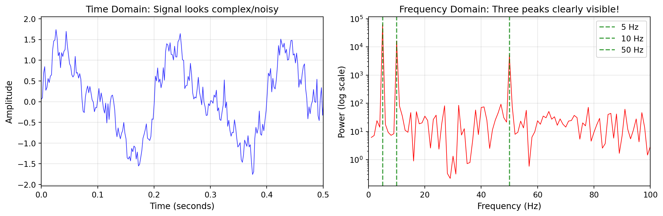
Visualizing the FFT: Time Domain vs Frequency Domain
The power of the FFT becomes clear when visualized—patterns invisible in the time domain jump out in the frequency domain:
Left: Composite signal looks noisy in time domain. Right: FFT reveals the three frequency components clearly.
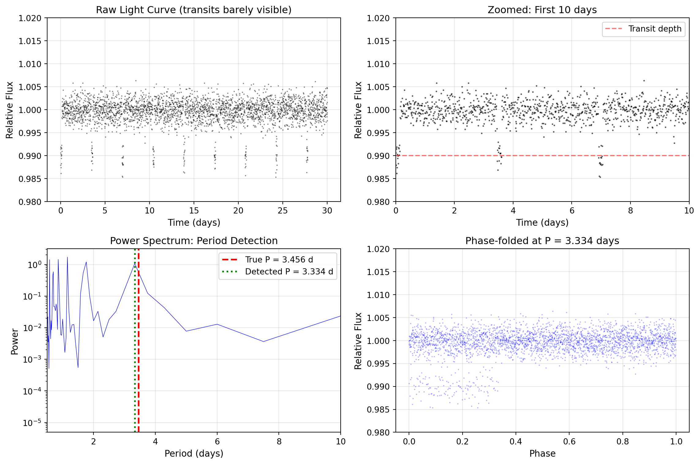
import numpy as npimport matplotlib.pyplot as plt# Practical example: Finding periodic signal in noisy data# Simulate exoplanet transit light curve with periodic dipstime = np.linspace(0, 30, 3000) # 30 days of observationsperiod =3.456# Planet orbital period in daystransit_duration =0.15# days# Create light curve with transitsflux = np.ones_like(time)phase = (time % period) / periodin_transit = phase < (transit_duration / period)flux[in_transit] *=0.99# 1% transit depth# Add realistic noiserng = np.random.default_rng(42)flux += rng.normal(0, 0.002, len(time)) # 0.2% noise# FFT to find periodicityfft_flux = np.fft.fft(flux - flux.mean()) # Remove DC componentfreqs_flux = np.fft.fftfreq(len(time), time[1] - time[0]) # Frequencies in 1/day# Power spectrumpower_flux = np.abs(fft_flux)**2# Look for peak in physically reasonable range (periods from 2 to 15 days)# Note: We use a narrower frequency range to avoid harmonics from the box-shaped transitfreq_mask = (freqs_flux >0.07) & (freqs_flux <0.5) # Periods ~2-14 dayspeak_freq = freqs_flux[freq_mask][np.argmax(power_flux[freq_mask])]detected_period =1/ peak_freqprint(f"True period: {period:.3f} days")print(f"Detected period: {detected_period:.3f} days")print(f"Error: {abs(detected_period - period)*24*60:.1f} minutes")# Visualize the transit detectionfig, axes = plt.subplots(2, 2, figsize=(12, 8))# Raw light curveaxes[0, 0].plot(time, flux, 'k.', markersize=1, alpha=0.5)axes[0, 0].set_xlabel('Time (days)', fontsize=11)axes[0, 0].set_ylabel('Relative Flux', fontsize=11)axes[0, 0].set_title('Raw Light Curve (transits barely visible)', fontsize=12)axes[0, 0].set_ylim(0.98, 1.02)axes[0, 0].grid(True, alpha=0.3)# Zoomed view showing transitsaxes[0, 1].plot(time, flux, 'k.', markersize=2, alpha=0.5)axes[0, 1].set_xlabel('Time (days)', fontsize=11)axes[0, 1].set_ylabel('Relative Flux', fontsize=11)axes[0, 1].set_title('Zoomed: First 10 days', fontsize=12)axes[0, 1].set_xlim(0, 10)axes[0, 1].set_ylim(0.98, 1.02)axes[0, 1].axhline(y=0.99, color='red', linestyle='--', alpha=0.5, label='Transit depth')axes[0, 1].legend()axes[0, 1].grid(True, alpha=0.3)# Power spectrumpos_freq_mask = freqs_flux >0axes[1, 0].semilogy(1/freqs_flux[pos_freq_mask], power_flux[pos_freq_mask], 'b-', linewidth=0.5)axes[1, 0].axvline(x=period, color='red', linestyle='--', linewidth=2, label=f'True P = {period:.3f} d')axes[1, 0].axvline(x=detected_period, color='green', linestyle=':', linewidth=2, label=f'Detected P = {detected_period:.3f} d')axes[1, 0].set_xlabel('Period (days)', fontsize=11)axes[1, 0].set_ylabel('Power', fontsize=11)axes[1, 0].set_title('Power Spectrum: Period Detection', fontsize=12)axes[1, 0].set_xlim(0.5, 10)axes[1, 0].legend()axes[1, 0].grid(True, alpha=0.3)# Phase-folded light curvephase_fold = (time % detected_period) / detected_periodaxes[1, 1].plot(phase_fold, flux, 'b.', markersize=1, alpha=0.3)axes[1, 1].set_xlabel('Phase', fontsize=11)axes[1, 1].set_ylabel('Relative Flux', fontsize=11)axes[1, 1].set_title(f'Phase-folded at P = {detected_period:.3f} days', fontsize=12)axes[1, 1].set_ylim(0.98, 1.02)axes[1, 1].grid(True, alpha=0.3)plt.tight_layout()plt.show()
True period: 3.456 days
Detected period: 3.334 days
Error: 175.0 minutes
FFT detection of exoplanet transit period from noisy light curve data
Reality check: FFTs are excellent for sinusoidal signals, but transit light curves are boxy and generate strong harmonics. In practice, astronomers often use Box Least Squares (BLS) for transit searches and Lomb–Scargle periodograms for unevenly sampled data. You do not need those methods yet — just know that FFT is a first look, not the final word.
Tip💡 Advanced: Window Functions and Spectral Leakage
When your signal doesn’t fit perfectly within your sampling window (which is almost always!), the FFT produces spectral leakage — power spreads to neighboring frequencies, creating artificial peaks.
Window functions reduce this leakage by tapering the signal edges. Common choices include:
Hanning (np.hanning(N)): Good general-purpose choice, reduces leakage significantly
Hamming (np.hamming(N)): Similar to Hanning, slightly different sidelobe structure
Blackman (np.blackman(N)): Best sidelobe suppression, wider main lobe
# Apply a window function before FFTwindow = np.hanning(len(signal))windowed_signal = signal * windowfft_windowed = np.fft.fft(windowed_signal)
For this course, you won’t need window functions — but knowing they exist prepares you for advanced signal processing!
NoteQuick Check
If your sampling rate doubles while your number of samples stays the same, what happens to the Nyquist frequency and the frequency resolution?
Covariance and Correlation
Covariance and correlation measure how two variables change together – crucial for understanding relationships in astronomical data like the color-magnitude diagram, period-luminosity relations, or Tully-Fisher correlations.
\(\mu_X\), \(\mu_Y\) (or \(\bar{x}\), \(\bar{y}\)) are the means of \(X\) and \(Y\)
\(n\) is the number of data points
Interpretation:
Positive covariance: Variables tend to increase together
Negative covariance: When one increases, the other tends to decrease
Zero covariance: No linear relationship (but there could be nonlinear relationships!)
Problem with covariance: It depends on the units. Temperature in Kelvin vs Celsius gives different covariances with luminosity! The units of covariance are the units of \(X\) multiplied by the units of \(Y\), which makes raw covariance hard to compare across unit systems. For sample covariance, you often divide by \(n-1\) instead of \(n\); np.cov uses the \(n-1\) convention by default.
Correlation coefficient (Pearson’s \(r\)) solves this by normalizing:
\[
r = \frac{\mathrm{Cov}(X,Y)}{\sigma_X\sigma_Y}
\]
Where \(\sigma_X\) and \(\sigma_Y\) are the standard deviations. This gives:
\(r \in [-1, 1]\) always
\(r = 1\): Perfect positive linear correlation
\(r = -1\): Perfect negative linear correlation
\(r = 0\): No linear correlation
\(|r| > 0.7\): Generally considered strong correlation
\(|r| < 0.3\): Generally considered weak correlation
Covariance Matrix:
For multiple variables, we organize covariances into a matrix:
       X    Y    Z
   X  Var(X) Cov(X,Y) Cov(X,Z)
   Y  Cov(Y,X) Var(Y) Cov(Y,Z)
   Z  Cov(Z,X) Cov(Z,Y) Var(Z)
The diagonal contains variances (a variable’s covariance with itself), and the matrix is symmetric (\(\mathrm{Cov}(X,Y) = \mathrm{Cov}(Y,X)\)).
# Calculate covariance and correlation between datasets# Simulate correlated stellar propertiesrng = np.random.default_rng(42)n_stars =100temperature = rng.normal(5800, 500, n_stars) # Kelvin# Luminosity correlates with temperature (Stefan-Boltzmann: L propto T^4)# Add noise to make it realisticluminosity_true = (temperature/5800)**4# Normalized to solarluminosity = luminosity_true + rng.normal(0, 0.1, n_stars)# Manual calculation to understand the mathtemp_mean = temperature.mean()lum_mean = luminosity.mean()temp_centered = temperature - temp_meanlum_centered = luminosity - lum_mean# Covariance: average of products of deviationscovariance_manual = (temp_centered * lum_centered).mean()print(f"Manual covariance: {covariance_manual:.6f}")# Standard deviationstemp_std = temperature.std()lum_std = luminosity.std()# Correlation coefficientcorrelation_manual = covariance_manual / (temp_std * lum_std)print(f"Manual correlation: {correlation_manual:.3f}")# Using NumPy functions# Covariance matrixcov_matrix = np.cov(temperature, luminosity)print(f"\nCovariance matrix:\n{cov_matrix}")print(f"Temperature variance: {cov_matrix[0,0]:.1f}")print(f"Luminosity variance: {cov_matrix[1,1]:.6f}")print(f"Temp-Lum covariance: {cov_matrix[0,1]:.6f}")# Correlation coefficientcorr_matrix = np.corrcoef(temperature, luminosity)print(f"\nCorrelation matrix:\n{corr_matrix}")print(f"Correlation coefficient: {corr_matrix[0,1]:.3f}")# Interpretationifabs(corr_matrix[0,1]) >0.7: strength ="strong"elifabs(corr_matrix[0,1]) >0.3: strength ="moderate"else: strength ="weak"print(f"This indicates a {strength} correlation between temperature and luminosity")
# Multiple variables: complete covariance analysis# Add more stellar propertiesrng = np.random.default_rng(42)mass = rng.normal(1, 0.3, n_stars) # Solar masses# Radius correlates with mass (mass-radius relation)radius = mass**0.8+ rng.normal(0, 0.05, n_stars)# Age (uncorrelated with current properties for main sequence)age = rng.uniform(1, 10, n_stars) # Gyr# Stack all variablesdata = np.vstack([temperature, luminosity, mass, radius, age])# Full covariance matrixfull_cov = np.cov(data)print("Full covariance matrix shape:", full_cov.shape)# Full correlation matrix (easier to interpret)full_corr = np.corrcoef(data)labels = ['Temp', 'Lum', 'Mass', 'Radius', 'Age']print("\nCorrelation matrix:")print(" ", " ".join(f"{l:>7}"for l in labels))for i, label inenumerate(labels):print(f"{label:>7}", " ".join(f"{full_corr[i,j]:7.3f}"for j inrange(5)))print("\nStrong correlations (|r| > 0.5):")for i inrange(5):for j inrange(i+1, 5):ifabs(full_corr[i,j]) >0.5:print(f" {labels[i]}-{labels[j]}: {full_corr[i,j]:.3f}")
# Cross-correlation for time series alignment# Useful for aligning light curves or spectrasignal1 = np.sin(np.linspace(0, 10, 100))signal2 = np.sin(np.linspace(0, 10, 100) +1) # Phase shifted# Cross-correlation finds the shiftcorrelation = np.correlate(signal1, signal2, mode='same')lag = np.argmax(correlation) -len(correlation)//2print(f"Maximum correlation at lag: {lag} samples")# This tells us signal2 is shifted relative to signal1
Important🌟 Why This Matters: The Vera Rubin Observatory’s Data Challenge
The Vera Rubin Observatory (formerly LSST) will produce enormous data volumes every night. Using Python lists instead of NumPy arrays would make this impossible.
Astro example — the same memory and throughput issues appear in satellite imaging, genomics, and materials characterization.
Memory Requirements: Python lists store objects with large overhead, while NumPy stores contiguous numeric buffers. For large images with millions of pixels, lists can be orders of magnitude larger than arrays.
Processing Speed: Detecting moving asteroids requires comparing images pixel-by-pixel. Vectorized NumPy operations make those comparisons fast enough to be practical.
Real-time Alerts: NumPy’s speed enables rapid detection and alerting for transient events — the core workflow of time-domain astronomy.
Without NumPy’s memory efficiency and speed, modern time-domain astronomy would be infeasible. The same library you’re learning makes it possible to monitor the sky for changes every night.
Let’s create concrete performance benchmarks you can run on your system:
"""Performance comparison: Lists vs NumPyRun these on your machine - results vary by hardware!"""import timeimport numpy as npdef benchmark_operation(name, list_func, numpy_func, size=100000):"""Benchmark a single operation."""# Setup data list_data =list(range(size)) numpy_data = np.arange(size, dtype=float)# Time list operation start = time.perf_counter() list_result = list_func(list_data) list_time = time.perf_counter() - start# Time NumPy operation start = time.perf_counter() numpy_result = numpy_func(numpy_data) numpy_time = time.perf_counter() - start speedup = list_time / numpy_timereturn list_time *1000, numpy_time *1000, speedup# Define operations to benchmarkoperations = {"Element-wise square": (lambda x: [i**2for i in x],lambda x: x**2 ),"Sum all elements": (lambda x: sum(x),lambda x: x.sum() ),"Element-wise sqrt": (lambda x: [i**0.5for i in x],lambda x: np.sqrt(x) ),"Find maximum": (lambda x: max(x),lambda x: x.max() )}print("Performance Comparison (100,000 elements):")print("-"*60)print(f"{'Operation':<20}{'List (ms)':<12}{'NumPy (ms)':<12}{'Speedup':<10}")print("-"*60)for name, (list_op, numpy_op) in operations.items(): list_ms, numpy_ms, speedup = benchmark_operation(name, list_op, numpy_op)print(f"{name:<20}{list_ms:<12.2f}{numpy_ms:<12.3f}{speedup:<10.1f}x")
import timeimport numpy as np# Matrix multiplication comparison (smaller size due to O(n^3) complexity)def matrix_multiply_lists(A, B):"""Matrix multiplication with nested lists.""" n =len(A) C = [[0]*n for _ inrange(n)]for i inrange(n):for j inrange(n):for k inrange(n): C[i][j] += A[i][k] * B[k][j]return C# Create test matricesn =100# 100x100 matricesA_list = [[float(i+j) for j inrange(n)] for i inrange(n)]B_list = [[float(i-j) for j inrange(n)] for i inrange(n)]A_numpy = np.array(A_list)B_numpy = np.array(B_list)# Benchmark matrix multiplicationstart = time.perf_counter()C_list = matrix_multiply_lists(A_list, B_list)list_matmul_time = time.perf_counter() - startstart = time.perf_counter()C_numpy = A_numpy @ B_numpynumpy_matmul_time = time.perf_counter() - startprint(f"\nMatrix Multiplication (100x100):")print(f" Nested loops: {list_matmul_time*1000:.1f} ms")print(f" NumPy (@): {numpy_matmul_time*1000:.3f} ms")print(f" Speedup: {list_matmul_time/numpy_matmul_time:.0f}x")
Note🔍 Check Your Understanding
Why is np.empty() faster than np.zeros() but potentially dangerous?
TipAnswer
np.empty() allocates memory without initializing values, while np.zeros() allocates and sets all values to 0.
# empty is faster but contains garbageempty_arr = np.empty(5)print(empty_arr) # Random values from memory!# zeros is slower but safezero_arr = np.zeros(5)print(zero_arr) # Guaranteed [0. 0. 0. 0. 0.]
Use np.empty() only when you’ll immediately overwrite all values. Otherwise, you might accidentally use uninitialized data, leading to non-reproducible bugs!
NumPy Gotchas: Top 5 Student Mistakes
Warning⚠️ Common NumPy Pitfalls
Integer division with integer arrays
# Wrong: integer divisionarr = np.array([1, 2, 3])normalized = arr / arr.max() # Works but be careful with //# Safe: always use floats for sciencearr = np.array([1, 2, 3], dtype=float)
Views modify the original
data = np.arange(10)view = data[2:8]view[0] =999# Changes data[2] to 999!
You’ve just acquired the fundamental tool that transforms Python into a scientific computing powerhouse. NumPy isn’t just a faster way to work with numbers – it’s a different way of thinking about computation. Instead of writing loops that process elements one at a time, you now express mathematical operations on entire datasets at once. This vectorized thinking mirrors how we conceptualize scientific problems: we don’t think about individual photons hitting individual pixels; we think about images, spectra, and light curves as coherent wholes. NumPy lets you write code that matches this conceptual model, making your programs both faster and more readable.
The performance gains you’ve witnessed aren’t just convenient; they’re transformative. Calculations that would be sluggish with Python lists can become fast with NumPy arrays. This speed isn’t achieved through complex optimization tricks but through NumPy’s elegant design: contiguous memory storage, vectorized operations that call optimized compiled routines, and broadcasting that eliminates redundant data copying. The same ideas that make your homework scripts faster also power large‑scale data analysis workflows at observatories and laboratories worldwide.
Beyond performance, NumPy provides a vocabulary for scientific computing that’s consistent across the entire Python ecosystem. The array indexing, broadcasting rules, and ufuncs you’ve learned aren’t just NumPy features – they’re the standard interface for numerical computation in Python. When you move on to using SciPy for optimization, Matplotlib for visualization, or Pandas for data analysis, you’ll find they all speak NumPy’s language. This consistency means the effort you’ve invested in understanding NumPy pays dividends across every scientific Python library you’ll ever use. You’ve learned to leverage views for memory efficiency, use boolean masking for sophisticated data filtering, and apply broadcasting to solve complex problems elegantly. These aren’t just programming techniques; they’re computational thinking patterns that will shape how you approach every numerical problem.
You’ve also mastered the random number generation capabilities essential for Monte Carlo simulations – a cornerstone of modern computational astrophysics. From simulating photon counting statistics with Poisson distributions to modeling measurement errors with Gaussian noise, you now have the tools to create realistic synthetic data and perform statistical analyses. The ability to generate random samples from various distributions, perform bootstrap resampling, and create correlated multivariate data will be crucial in your upcoming projects, especially when you tackle Monte Carlo sampling techniques.
Looking ahead, NumPy arrays will be the primary data structure for the rest of your scientific computing journey. Every image you process, every spectrum you analyze, every simulation you run will flow through NumPy arrays. You now have the tools to use NumPy for arrays and the math module for scalar-only tasks when appropriate. The concepts you’ve mastered – vectorization, broadcasting, boolean masking – aren’t just NumPy features; they’re the foundation of modern computational science. You’re no longer limited by Python’s native capabilities; you have access to the same computational power that enables large‑scale data analysis across many scientific fields. In the next chapter, you’ll see how NumPy arrays become the canvas for scientific visualization with Matplotlib, where every plot, image, and diagram starts with the arrays you now know how to create and manipulate.
NoteQuick Check
Suppose you want to compute the mean of each row of a 2D array and subtract it from that row. Which shape should the row means have to broadcast correctly?
Definitions
Array: NumPy’s fundamental data structure, a grid of values all of the same type, indexed by a tuple of integers.
Boolean Masking: Using an array of boolean values to select elements from another array that meet certain conditions.
Broadcasting: NumPy’s mechanism for performing operations on arrays of different shapes by automatically expanding dimensions according to specific rules.
CGS Units: Centimeter-Gram-Second unit system, traditionally used in astronomy and astrophysics for convenient scaling.
Contiguous Memory: Data stored in adjacent memory locations, enabling fast access and efficient cache utilization.
Copy: A new array with its own data, independent of the original array’s memory.
dtype: The data type of array elements, determining memory usage and numerical precision (e.g., float64, int32).
Monte Carlo: A computational technique using random sampling to solve problems that might be deterministic in principle.
ndarray: NumPy’s n-dimensional array object, the core data structure for numerical computation.
NumPy: Numerical Python, the fundamental package for scientific computing providing support for arrays and mathematical functions.
Shape: The dimensions of an array, given as a tuple indicating the size along each axis.
ufunc: Universal function, a NumPy function that operates element-wise on arrays, supporting broadcasting and type casting.
Universal Functions: NumPy functions that operate element-wise on arrays, supporting broadcasting and type casting.
Vectorization: Performing operations on entire arrays at once rather than using explicit loops, leveraging optimized C code.
View: A new array object that shares data with the original array, saving memory but linking modifications.
Key Takeaways
✔ NumPy arrays are often much faster than Python lists for numerical operations by using contiguous memory and calling optimized compiled routines
✔ Vectorization eliminates explicit loops by operating on entire arrays at once, making code both faster and more readable
✔ NumPy covers most math operations and adds array support – use np.sin() for arrays, and math for scalar-only work when appropriate
✔ Broadcasting enables operations on different-shaped arrays by automatically expanding dimensions, eliminating data duplication
✔ Boolean masking provides powerful data filtering using conditions to select array elements, essential for data analysis
✔ Essential creation functions like linspace, logspace, and meshgrid are workhorses for scientific computing
✔ Random number generation from various distributions (uniform, normal, Poisson) enables Monte Carlo simulations
✔ Memory layout matters – row-major vs column-major ordering can change performance
✔ Views share memory while copies are independent – understanding this prevents unexpected data modifications
✔ Array methods provide built-in analysis – .mean(), .std(), .max() operate efficiently along specified axes
✔ NumPy is the foundation of scientific Python – every major package (SciPy, Matplotlib, Pandas) builds on NumPy arrays
Quick Reference Tables
Array Creation Functions
Function
Purpose
Example
np.array()
Create from list
np.array([1, 2, 3])
np.zeros()
Initialize with 0s
np.zeros((3, 4))
np.ones()
Initialize with 1s
np.ones((2, 3))
np.empty()
Uninitialized (fast)
np.empty(5)
np.full()
Fill with value
np.full((3, 3), 7)
np.eye()
Identity matrix
np.eye(4)
np.arange()
Like Python’s range
np.arange(0, 10, 2)
np.linspace()
N evenly spaced
np.linspace(0, 1, 11)
np.logspace()
Log-spaced values
np.logspace(0, 3, 4)
np.meshgrid()
2D coordinate grids
np.meshgrid(x, y)
Essential Array Operations
Operation
Description
Example
+, -, *, /
Element-wise arithmetic
a + b
**
Element-wise power
a ** 2
//
Floor division
a // 2
%
Modulo
a % 3
@
Matrix multiplication
a @ b
np.dot()
Dot product
np.dot(a, b)
==, !=, <, >
Element-wise comparison
a > 5
&, |, ~
Boolean operations
(a > 0) & (a < 10)
.T
Transpose
matrix.T
.reshape()
Change dimensions
arr.reshape(3, 4)
.flatten()
Convert to 1D
matrix.flatten()
Statistical Methods
Method
Description
Example
.mean()
Average
arr.mean() or arr.mean(axis=0)
.std()
Standard deviation
arr.std()
.min()/.max()
Extrema
arr.min()
.sum()
Sum elements
arr.sum()
.cumsum()
Cumulative sum
arr.cumsum()
.argmin()/.argmax()
Index of extrema
arr.argmax()
np.median()
Median value
np.median(arr)
np.percentile()
Percentiles
np.percentile(arr, 95)
np.cov()
Covariance matrix
np.cov(x, y)
np.corrcoef()
Correlation coefficient
np.corrcoef(x, y)
np.histogram()
Compute histogram
np.histogram(data, bins=20)
Random Number Functions
Assume rng = np.random.default_rng(42) for the examples below.
Function
Distribution
Example
rng.uniform()
Uniform
rng.uniform(0, 1, 1000)
rng.random()
Uniform [0,1)
rng.random(100)
rng.normal()
Gaussian/Normal
rng.normal(0, 1, 1000)
rng.standard_normal()
Standard normal
rng.standard_normal(100)
rng.poisson()
Poisson
rng.poisson(100, 1000)
rng.exponential()
Exponential
rng.exponential(1.0, 1000)
rng.choice()
Random selection
rng.choice(arr, 10)
rng.permutation()
Shuffle array
rng.permutation(arr)
np.random.default_rng()
Create generator
rng = np.random.default_rng(42)
rng.multivariate_normal()
Multivariate normal
rng.multivariate_normal(mean, cov, n)
Common NumPy Functions
Function
Purpose
Math Equivalent
np.sin()
Sine
math.sin()
np.cos()
Cosine
math.cos()
np.exp()
Exponential
math.exp()
np.log()
Natural log
math.log()
np.log10()
Base-10 log
math.log10()
np.sqrt()
Square root
math.sqrt()
np.abs()
Absolute value
abs()
np.round()
Round to integer
round()
np.where()
Conditional selection
N/A
np.clip()
Bound values
N/A
np.unique()
Find unique values
set()
np.concatenate()
Join arrays
+ for lists
np.gradient()
Numerical derivative
N/A
np.interp()
Linear interpolation
N/A
np.allclose()
Float comparison
N/A
np.isnan()
Check for NaN
N/A
np.isinf()
Check for infinity
N/A
np.isfinite()
Check for finite
N/A
np.correlate()
Cross-correlation
N/A
Memory and Performance Reference
Operation
Returns View
Returns Copy
Basic slicing arr[2:8]
✓
Fancy indexing arr[[1,3,5]]
✓
Boolean masking arr[arr>5]
✓
.reshape()
✓
.flatten()
✓
.ravel()
✓ (usually)
.T or .transpose()
✓
Arithmetic arr + 1
✓
.copy()
✓
References
Harris, C. R., et al. (2020). Array programming with NumPy. Nature, 585(7825), 357-362.
van der Walt, S., Colbert, S. C., & Varoquaux, G. (2011). The NumPy array: a structure for efficient numerical computation. Computing in Science & Engineering, 13(2), 22-30.
Oliphant, T. E. (2006). A guide to NumPy. USA: Trelgol Publishing.
VanderPlas, J. (2016). Python Data Science Handbook. O’Reilly Media.
Johansson, R. (2019). Numerical Python: Scientific Computing and Data Science Applications with Numpy, SciPy and Matplotlib (2nd ed.). Apress.
Next Chapter Preview
In Chapter 8: Matplotlib - Visualizing Your Universe, you’ll discover how to transform the NumPy arrays you’ve mastered into publication-quality visualizations. You’ll learn to create everything from simple line plots to complex multi-panel figures displaying astronomical data. Using the same NumPy arrays you’ve been working with, you’ll visualize spectra with proper wavelength scales, create color-magnitude diagrams from stellar catalogs, display telescope images with world coordinate systems, and generate the kinds of plots that appear in research papers. You’ll master customization techniques to control every aspect of your figures, from axis labels with LaTeX formatting to colormaps optimized for astronomical data. The NumPy operations you’ve learned – slicing for zooming into data, masking for highlighting specific objects, and meshgrid for creating coordinate systems – become the foundation for creating compelling scientific visualizations. Most importantly, you’ll understand how NumPy and Matplotlib work together as an integrated system, with NumPy handling the computation and Matplotlib handling the visualization, forming the core workflow that will carry you through your entire career in computational astrophysics!