Part 2: Numbers Aren’t Real - Computer Arithmetic & Cosmic Consequences
Module 1: Foundations of Discrete Computing | COMP 536
Author
Anna Rosen
Mathematics treats real numbers as continuous and exact; computers store finite binary approximations. Numerical science begins when those worlds stop agreeing.
NoteOpening Prediction
Before the reading explains anything, decide what you expect from the familiar check 0.1 + 0.2 == 0.3.
If your first instinct is “of course that should be True,” keep that prediction in view. Part 2 is about why that instinct fails, and why the failure matters scientifically.
Learning Objectives
By the end of this section, you will be able to:
Why This Matters for Astronomy
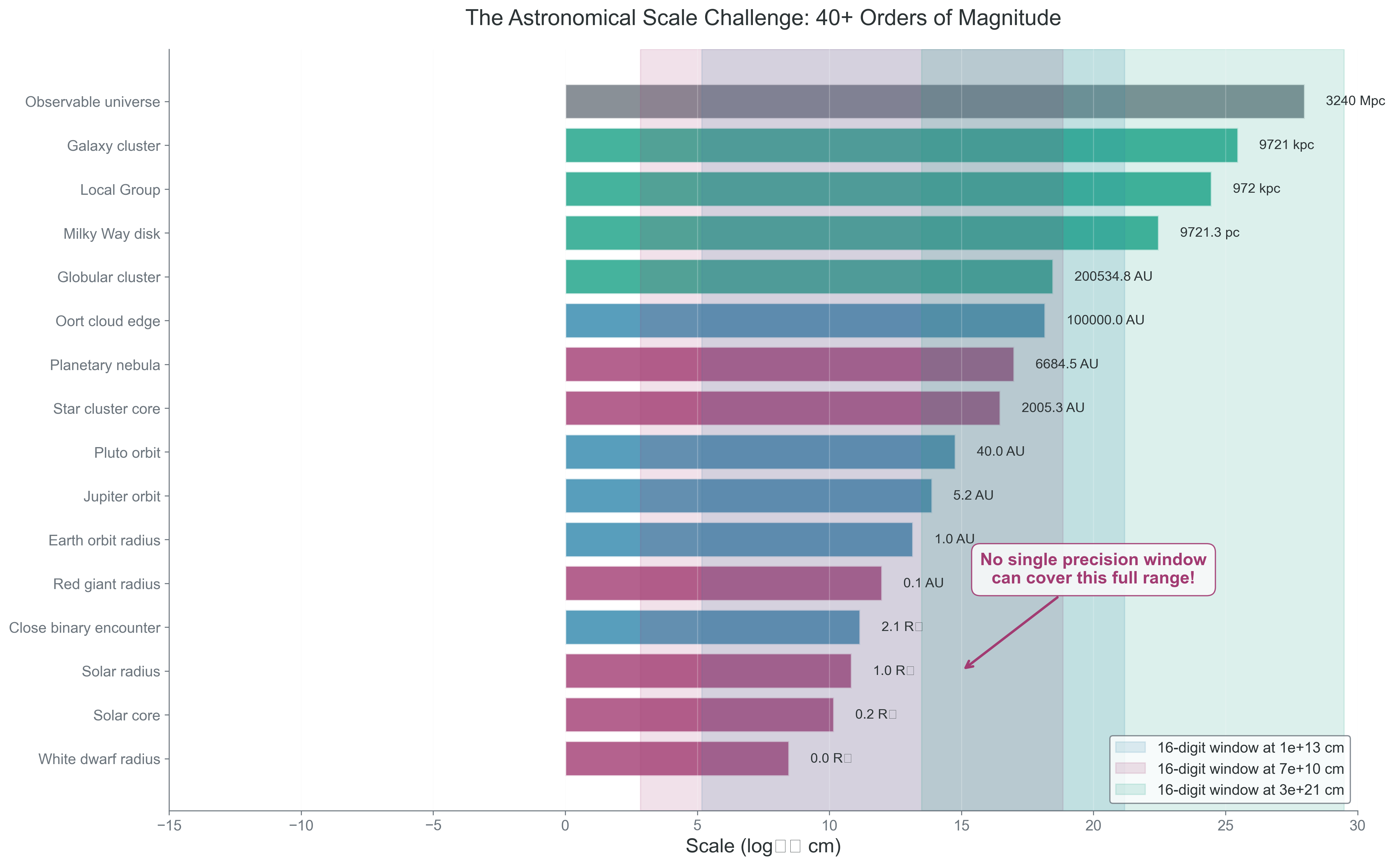
Why this matters: astronomy forces us to compute across enormous ranges of scale, and floating-point arithmetic does not adapt its precision automatically to the physics we care about.
Student mental model: the computer does not store “the real number.” It stores the nearest representable binary value. That approximation is often excellent, but when we subtract nearly equal numbers, span many orders of magnitude, or iterate millions of times, the approximation can shape the science.
Astronomical simulations routinely cross very different physical scales:
Mercury orbits at \(0.39\,\mathrm{AU}\), while Neptune orbits at \(30\,\mathrm{AU}\).
A molecular cloud may span \(\sim 10\,\mathrm{pc}\), while a protostellar core can be \(\sim 100\,\mathrm{AU}\).
A star-forming region might be \(\sim 1\,\mathrm{pc}\), while a galactic halo extends to \(\sim 100\,\mathrm{kpc}\).
which says that star-formation problems mix local structure and cloud-scale structure in the same calculation.
Double precision gives about 15 to 16 decimal digits of relative precision near numbers of order unity. That is an approximate practical statement about floating-point spacing, not a law of nature about “how many digits exist” in a calculation.
Figure 1: What to notice in this figure: the computational challenge is not just that astronomy spans many orders of magnitude. It is that no single coordinate scale makes every subtraction, normalization, and conservation check equally well conditioned.
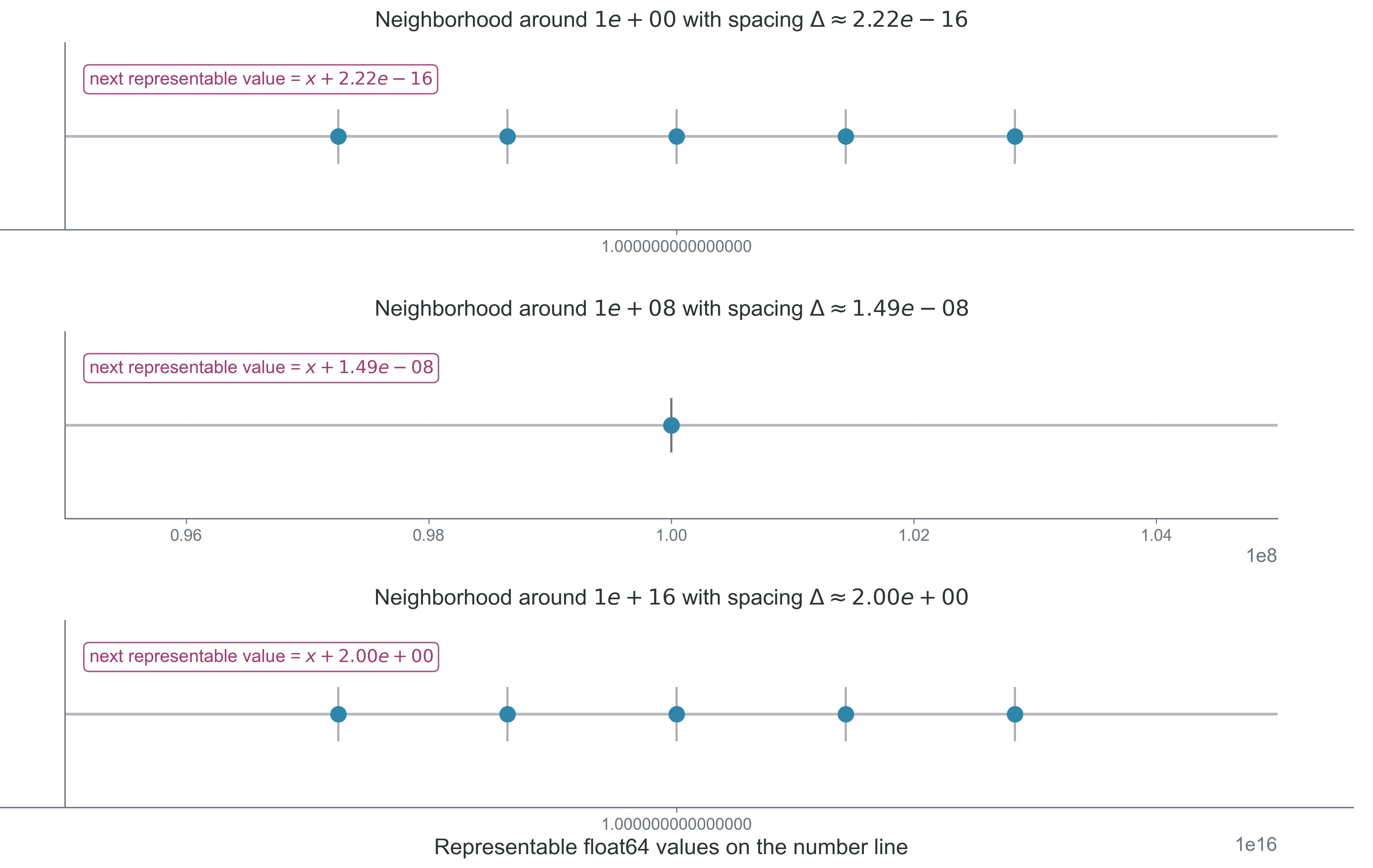
Figure 2: What to notice in this figure: representable numbers are discrete rather than continuous, and the gap between adjacent floating-point values grows with magnitude. That is why a subtraction that is safe near \(1\) may be ill-conditioned near \(10^{16}\).
The takeaway is that scale is part of the numerical problem. The same subtraction can be harmless at one magnitude and poorly conditioned at another.
Finding Machine Epsilon
Why this matters: machine epsilon is the local scale at which a floating-point number near \(1\) stops changing when you perturb it.
The standard definition is
\[
1 + \epsilon_{\mathrm{machine}} \neq 1.
\]
This equation says that \(\epsilon_{\mathrm{machine}}\) is the smallest positive floating-point number that still changes \(1\) when added to it.
This means that near numbers of order unity, relative perturbations much smaller than \(10^{-16}\) are typically invisible in double precision.
WarningCommon Misconception: Machine Epsilon Is Not a Universal Error Bound
\(\epsilon_{\mathrm{machine}}\) is not “the error in every calculation.” It is a local spacing scale near \(1\), and actual numerical error depends on magnitude, conditioning, algebraic form, and the sequence of operations.
Worked Example 1: Why 0.1 + 0.2 != 0.3
Why this matters: this is the simplest way to see that floating-point numbers are binary approximations, not exact decimal objects.
NotePrediction Before Calculation
Before running the code, predict the answer to this question: if Python stores decimal-looking numbers exactly, should 0.1 + 0.2 == 0.3 evaluate to True?
What quantity is being computed? - A Boolean equality test and the stored floating-point representations of 0.1, 0.2, and 0.3.
What is known exactly? - The mathematical decimal numbers \(0.1\), \(0.2\), and \(0.3\) are exact real numbers in base 10 notation.
What is represented approximately on the computer? - Their nearest binary floating-point approximations in double precision.
What does the error mean in practice? - Exact equality checks on floating-point numbers can fail even when the printed decimals look simple and familiar.
NoteCode Purpose
Purpose: expose the stored binary-floating-point approximations behind familiar decimal literals.
Inputs/Outputs: no user inputs; the code prints exact integer-ratio representations and comparison results.
Common pitfall: concluding that Python is “wrong” instead of recognizing that finite binary fractions cannot represent most finite decimals exactly.
Show the binary-representation surprise
def describe_float(value: float) ->tuple[int, int]:"""Return the exact numerator and denominator of a Python float."""return value.as_integer_ratio()values = [0.1, 0.2, 0.3, 0.1+0.2]for value in values: numerator, denominator = describe_float(value)print(f"value = {value!r:<20} stored as {numerator}/{denominator} "f"= {numerator / denominator:.17f}" )print(f"0.1 + 0.2 == 0.3 -> {(0.1+0.2) ==0.3}")print(f"0.1 + 0.2 -> {0.1+0.2:.17f}")print(f"0.3 -> {0.3:.17f}")
value = 0.1                  stored as 3602879701896397/36028797018963968 = 0.10000000000000001
value = 0.2                  stored as 3602879701896397/18014398509481984 = 0.20000000000000001
value = 0.3                  stored as 5404319552844595/18014398509481984 = 0.29999999999999999
value = 0.30000000000000004  stored as 1351079888211149/4503599627370496 = 0.30000000000000004
0.1 + 0.2 == 0.3 -> False
0.1 + 0.2        -> 0.30000000000000004
0.3              -> 0.29999999999999999
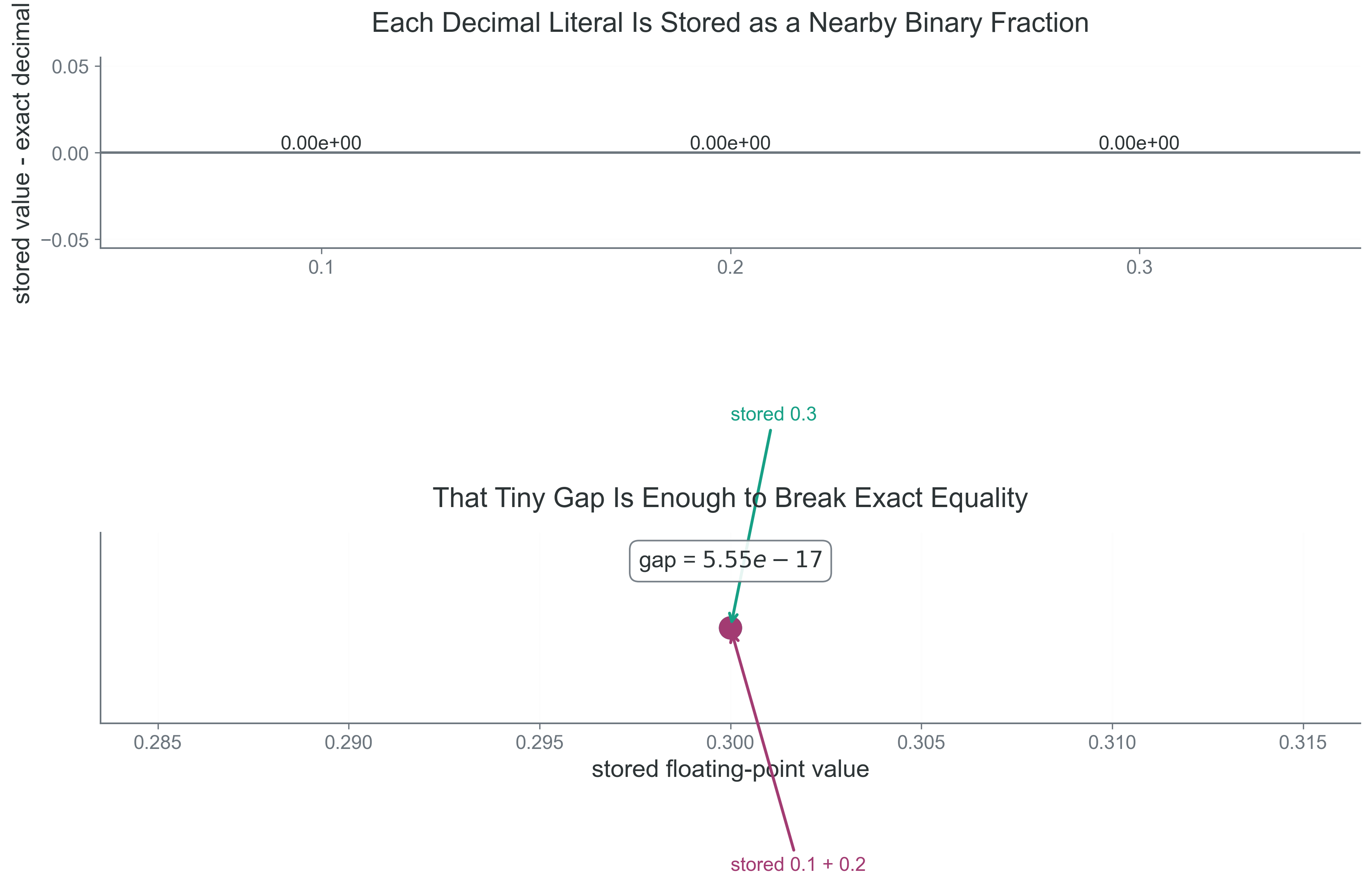
Interpretation: the mismatch is not folklore and it is not a Python bug. The finite binary approximation of \(0.1\) is slightly different from the exact real number \(0.1\), and those tiny differences survive arithmetic.
Figure 3: What to notice in this figure: the issue is not that the computer is careless. The issue is that most finite decimal fractions do not have finite binary expansions, so the stored values are the nearest available binary fractions.
Worked Example 2: Computing \(\epsilon_{\mathrm{machine}}\)
Why this matters: the abstract definition of machine epsilon becomes much easier to trust once you compute it yourself and compare it to NumPy’s built-in value.
NotePrediction Before Calculation
If the loop keeps halving a perturbation, do you expect the final answer to be exactly \(10^{-16}\), or only approximately of that order?
What quantity is being computed? - \(\epsilon_{\mathrm{machine}}\) for double precision.
What is known exactly? - NumPy reports the reference value through np.finfo(float).eps.
What is represented approximately on the computer? - Each trial perturbation in the halving loop is itself a floating-point number.
What does the error mean in practice? - This tells you the local relative spacing scale near \(1\), which is often the floor below which further refinement is pointless.
NoteCode Purpose
Purpose: compute machine epsilon with a loop and compare it with the library value.
Inputs/Outputs: no user inputs; the code returns one floating-point value and prints a consistency check.
Common pitfall: thinking the loop gives a universal tolerance for all numerical tasks. It only characterizes spacing near \(1\).
Interpretation: the loop and the library agree because both are describing the same hardware-level double-precision format. The result is approximately \(2.22\times 10^{-16}\), not exactly \(10^{-16}\), because binary floating-point spacing is not organized in decimal powers.
Machine epsilon is a local spacing scale, not a universal error budget.
The Three Types of Error
Why this matters: students often treat all numerical error as one fuzzy category, but different errors come from different causes and require different fixes.
Representation Error: Round-off Error
Why this matters: if the computer cannot represent a number exactly, error is present before your algorithm even begins.
Student mental model: round-off error is a storage problem. The value you wanted and the value the computer stores are nearby, but not identical.
We can write the local scale of round-off influence schematically as
This equation says that representation error is tied to floating-point spacing, though the proportionality constant depends strongly on the problem and the operation being performed.
Algorithmic Approximation Error: Truncation Error
Why this matters: even with exact arithmetic, many scientific algorithms intentionally approximate an infinite process with a finite one.
Student mental model: truncation error is an algorithm-design problem. You stop a series, discretize a derivative, or take a finite timestep, and that choice introduces approximation error.
For a method of order \(p\), a standard local model is
\[
E_{\mathrm{trunc}} \propto h^p.
\]
This equation says that the error decreases as the resolution parameter \(h\) shrinks, provided you are in the regime where the asymptotic model actually applies.
Accumulation and Amplification Error
Why this matters: a tiny per-step error can still become scientifically important if the computation repeats the step many times or amplifies perturbations dynamically.
Student mental model: propagation error is a history problem. The error you make now can be carried, accumulated, or magnified by everything that happens later.
If the signs of individual errors behave roughly like independent random kicks, a common model is
This equation says that random-sign accumulation behaves like a random walk, so the total error grows more slowly than linearly with the number of steps \(n\).
If the bias is coherent from step to step, a conservative model is
This equation says that systematic bias can accumulate linearly with the number of steps, which is much more dangerous for long integrations.
ImportantOne Computation Can Contain All Three
A finite-difference derivative in floating-point arithmetic can include all three error types at once:
representation error because numbers are stored approximately,
truncation error because the derivative formula is finite,
propagation or amplification error if the derivative is used repeatedly inside a larger algorithm.
The takeaway is that different error sources call for different fixes. Better algebra, better resolution, and better diagnostics solve different problems.
Catastrophic Cancellation
Why this matters: catastrophic cancellation is the signature failure mode of subtracting nearly equal numbers in floating-point arithmetic.
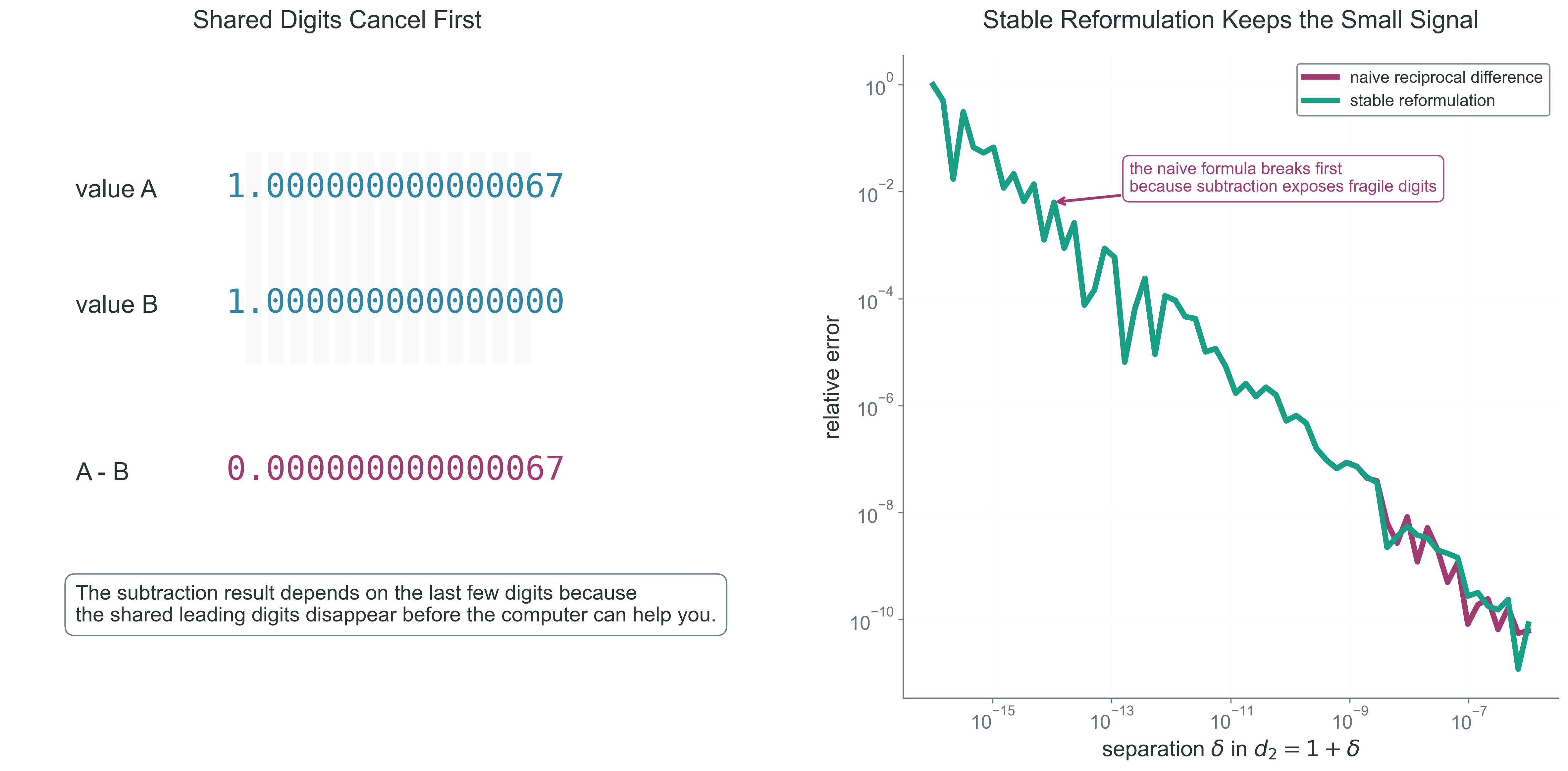
Student mental model: when two nearly equal numbers are subtracted, the leading digits cancel and the remaining digits may contain very little reliable information. The problem is not the subtraction itself; the problem is that the subtraction exposes the least accurate part of both inputs.
Worked Example 3: A Stable and Unstable Parallax-Like Difference
Why this matters: astronomy often asks us to compare nearby distances, inverse distances, or optical-depth-like quantities where the naive algebra is numerically brittle.
NotePrediction Before Calculation
If \(d_1\) and \(d_2\) are very close, which do you expect to be more stable numerically: \[
\frac{1}{d_1} - \frac{1}{d_2}
\quad \text{or} \quad
\frac{d_2-d_1}{d_1 d_2}\,?
\]
What quantity is being computed? - The difference between two inverse distances, measured here in \(\mathrm{AU}^{-1}\).
What is known exactly? - The two algebraic expressions are mathematically equivalent.
What is represented approximately on the computer? - The floating-point values of \(d_1\), \(d_2\), and their reciprocal evaluations.
What does the error mean in practice? - A naive formula can lose significant digits and make a small astrophysical signal look noisier or less trustworthy than it should.
NoteCode Purpose
Purpose: compare an unstable subtraction of reciprocals with a stable algebraic reformulation.
Inputs/Outputs: inputs are two positive distances; outputs are the naive value and the reformulated value in inverse-distance units.
Common pitfall: assuming two algebraically equivalent formulas are equally accurate in floating-point arithmetic.
Show the stable and unstable inverse-distance formulas
def _validate_positive_finite_distance(name: str, value: float) ->float:"""Validate a positive finite distance value.""" scalar =float(value)ifnot np.isfinite(scalar) or scalar <=0.0:raiseValueError(f"{name} must be a positive finite distance.")return scalardef parallax_bad(d1: float, d2: float) ->float:"""Return a naive difference of reciprocals.""" d1_checked = _validate_positive_finite_distance("d1", d1) d2_checked = _validate_positive_finite_distance("d2", d2)return1.0/ d1_checked -1.0/ d2_checkeddef parallax_good(d1: float, d2: float) ->float:"""Return the algebraically equivalent but numerically safer form.""" d1_checked = _validate_positive_finite_distance("d1", d1) d2_checked = _validate_positive_finite_distance("d2", d2)return (d2_checked - d1_checked) / (d1_checked * d2_checked)
Interpretation: both formulas are correct algebraically, but the stable form postpones the dangerous subtraction until after the denominator has been formed. The point is not that every toy example explodes dramatically in absolute error. The point is that one formula preserves more trustworthy significant digits than the other.
Show the lost-digit comparison against a high-precision reference
Interpretation: the stable formula is not “more correct” algebraically. It is more trustworthy numerically because it spends fewer significant digits before you reach the small signal you care about.
Stable Reformulation
Why this matters: when a numerical expression is fragile, the first fix is often algebraic rather than algorithmic.
Another classic example is
\[
\frac{a^2-b^2}{a-b} = a+b.
\]
This equation says that if \(a\) and \(b\) are close, the left-hand side performs two unstable operations before dividing, while the right-hand side avoids the cancellation entirely.
WarningDebugging Intuition
If a quantity should be small because of physics, do not assume a noisy result is “just a small signal.” Ask whether you are subtracting two large nearly equal numbers to get it.
Figure 4: What to notice in this figure: the dangerous step is not “small minus small.” It is “almost equal minus almost equal,” because the shared leading digits cancel and expose the least reliable trailing digits.
Algebraic equivalence does not imply numerical equivalence. Catastrophic cancellation is a conditioning problem exposed by subtraction.
Measuring Errors: Absolute vs. Relative
Why this matters: the same numerical difference can be negligible in one context and catastrophic in another.
This equation measures the discrepancy relative to the size of the true value, which is often more meaningful away from zero.
WarningCommon Misconception: Relative Error Is Not Always Better
Relative error is extremely useful when the true value is safely away from zero. Near zero, it can become misleading or undefined, and absolute error is often the more honest metric.
NoteCode Purpose
Purpose: compute absolute and relative error while handling near-zero regimes explicitly.
Inputs/Outputs: inputs are a computed value, a true value, and an optional problem scale for deciding when “near zero” matters; output is a dictionary of error diagnostics.
Common pitfall: reporting only relative error for a quantity whose physically meaningful scale is close to zero.
Show the error-metric helper
def absolute_relative_error( computed: float, true: float, zero_scale: float|None=None,) ->dict[str, float|str]:"""Return absolute and relative error with a near-zero decision rule.""" computed_scalar =float(computed) true_scalar =float(true)ifnot np.isfinite(computed_scalar) ornot np.isfinite(true_scalar):raiseValueError("computed and true must both be finite.")if zero_scale isnotNone: zero_scale_scalar =float(zero_scale)ifnot np.isfinite(zero_scale_scalar) or zero_scale_scalar <=0.0:raiseValueError("zero_scale must be a positive finite value when provided.")else: zero_scale_scalar =1.0 absolute_error =abs(computed_scalar - true_scalar) near_zero_threshold = np.sqrt(np.finfo(float).eps) * zero_scale_scalarifabs(true_scalar) <= near_zero_threshold: relative_error = math.nan recommended_metric ="absolute"else: relative_error = absolute_error /abs(true_scalar) recommended_metric ="relative"return {"absolute_error": absolute_error,"relative_error": relative_error,"recommended_metric": recommended_metric,"near_zero_threshold": near_zero_threshold, }
Worked Example 4: Computing Jupiter’s Mass
Why this matters: a large absolute difference can still be an excellent result if the reference quantity is enormous.
NotePrediction Before Calculation
If the computed mass differs from the true mass by \(10^{27}\,\mathrm{g}\), do you expect the result to be scientifically terrible or possibly quite good?
What quantity is being computed? - The error in a computed value of Jupiter’s mass.
What is known exactly? - For this worked example, we take the reference value \[
M_{\mathrm{true}} = 1.898\times 10^{30}\,\mathrm{g}
\] as the accepted true value.
What is represented approximately on the computer? - The computed value \[
M_{\mathrm{computed}} = 1.897\times 10^{30}\,\mathrm{g}.
\]
What does the error mean in practice? - It shows how absolute and relative error can tell very different stories about the same numerical result.
Absolute error: 1.000e+27 g
Relative error: 5.269e-04
Recommended metric: relative
Interpretation: the absolute error is physically large because Jupiter is physically large. The relative error is the better summary here because the true value is nowhere near zero.
Worked Example 5: Near-Zero Failure of Relative Error
Why this matters: near zero, relative error can look dramatic even when the physical discrepancy is negligible.
NotePrediction Before Calculation
If the true center-of-mass velocity is almost zero, would you rather know the fractional error or the absolute velocity offset in \(\mathrm{cm\,s^{-1}}\)?
What quantity is being computed? - The error in a nearly zero center-of-mass radial velocity.
What is known exactly? - For this worked example, we take \[
v_{\mathrm{true}} = 1.0\times 10^{-8}\,\mathrm{cm\,s^{-1}}
\] as the reference value.
What is represented approximately on the computer? - The computed value \[
v_{\mathrm{computed}} = 2.0\times 10^{-8}\,\mathrm{cm\,s^{-1}}.
\]
What does the error mean in practice? - The relative error is \(100\%\), but the physical mismatch is only \(10^{-8}\,\mathrm{cm\,s^{-1}}\), which may be negligible in a large simulation.
Show the near-zero error example
v_true =1.0e-8# cm s^-1v_computed =2.0e-8# cm s^-1velocity_errors = absolute_relative_error(v_computed, v_true, zero_scale=1.0e5)print(f"Absolute error: {velocity_errors['absolute_error']:.3e} cm s^-1")print(f"Relative error: {velocity_errors['relative_error']:.3e}")print(f"Recommended metric: {velocity_errors['recommended_metric']}")
Absolute error:      1.000e-08 cm s^-1
Relative error:      nan
Recommended metric:  absolute
Interpretation: the relative error sounds catastrophic because the denominator is tiny. In practice, the absolute error may be the more meaningful diagnostic when the physically relevant baseline is close to zero.
Show the regime comparison for absolute and relative error
import matplotlib.pyplot as pltregime_names = ["large quantity", "moderate quantity", "near-zero quantity"]true_values = np.array([1.898e30, 1.0, 1.0e-8])computed_values = np.array([1.897e30, 0.95, 2.0e-8])absolute_errors = np.abs(computed_values - true_values)relative_errors = absolute_errors / np.abs(true_values)fig, axes = plt.subplots(2, 1, figsize=(8.5, 5.8), sharex=True)x_positions = np.arange(len(regime_names))palette = [plt.get_cmap("tab10")(idx) for idx inrange(len(regime_names))]axes[0].plot(x_positions, absolute_errors, marker="o", linewidth=2.0, color=palette[0])axes[0].set_yscale("log")axes[0].set_ylabel(r"$E_{\mathrm{abs}}$")axes[0].set_title("Absolute error across three regimes")axes[1].plot(x_positions, relative_errors, marker="s", linewidth=2.0, color=palette[1])axes[1].set_yscale("log")axes[1].set_ylabel(r"$E_{\mathrm{rel}}$")axes[1].set_title("Relative error across the same three regimes")axes[1].set_xticks(x_positions, regime_names, rotation=15)for ax in axes: ax.grid(True, axis="y", alpha=0.25)fig.tight_layout()plt.show()
What to notice: the large-scale and moderate-scale cases keep relative error in its natural role as a size-aware summary, while the near-zero case breaks that intuition. The point is not that relative error is bad, but that it becomes misleading when the reference value nearly vanishes.
Relative error is powerful away from zero and often misleading near zero.
Tracking Accumulated Error
Why this matters: long-running simulations care not just about per-step error, but about what happens to those errors after thousands, millions, or billions of updates.
Worked Example 6: Error Propagation Over Many Steps
Why this matters: repeated updates can turn an individually tiny error into a meaningful drift.
NotePrediction Before Calculation
If a calculation carries a tiny coherent bias at every step, do you expect the total error to grow more like \(\sqrt{n}\) or more like \(n\)?
What quantity is being computed? - Model accumulated error after repeated updates.
What is known exactly? - We prescribe the per-step error model rather than measuring a hidden true trajectory.
What is represented approximately on the computer? - The cumulative effect of small errors over many steps.
What does the error mean in practice? - It tells you why long integrations require stronger diagnostics than one-step calculations.
NoteCode Purpose
Purpose: compare random-walk-like accumulation with coherent linear accumulation.
Inputs/Outputs: inputs are step counts and a per-step error scale; output is a list of dictionaries that can be printed, tested, or plotted.
Common pitfall: presenting one growth law as universal. Different algorithms and different problems can accumulate error in very different ways.
Show the error-propagation helper
def demonstrate_error_propagation( step_counts: Iterable[int], per_step_error: float= np.finfo(float).eps,) ->list[dict[str, float]]:"""Return random and systematic accumulation models for a set of step counts.""" per_step_error_scalar =float(per_step_error)ifnot np.isfinite(per_step_error_scalar) or per_step_error_scalar <=0.0:raiseValueError("per_step_error must be a positive finite number.") results: list[dict[str, float]] = []for step_count in step_counts: step_count_int =int(step_count)if step_count_int <=0:raiseValueError("All step counts must be positive integers.") random_walk_model = np.sqrt(step_count_int) * per_step_error_scalar systematic_model = step_count_int * per_step_error_scalar results.append( {"step_count": float(step_count_int),"random_walk_error": random_walk_model,"systematic_error": systematic_model, } )return results
Show the error-propagation example
propagation_results = demonstrate_error_propagation([1, 10, 100, 10_000, 1_000_000])for row in propagation_results:print(f"steps = {int(row['step_count']):>8d} "f"random model = {row['random_walk_error']:.3e} "f"systematic model = {row['systematic_error']:.3e}" )
steps =        1  random model = 2.220e-16  systematic model = 2.220e-16
steps =       10  random model = 7.022e-16  systematic model = 2.220e-15
steps =      100  random model = 2.220e-15  systematic model = 2.220e-14
steps =    10000  random model = 2.220e-14  systematic model = 2.220e-12
steps =  1000000  random model = 2.220e-13  systematic model = 2.220e-10
Interpretation: the random-walk model grows more slowly because positive and negative errors partially cancel. The systematic model grows faster because every step pushes in the same direction.
Figure 5: What to notice in this figure: random-sign accumulation and coherent bias do not threaten long integrations in the same way. The random-walk curve grows slowly, while the systematic curve grows much faster and can dominate long-running calculations.
The takeaway is that repeated tiny errors matter because history matters. Growth law, sign structure, and amplification all change the scientific risk.
Adaptive Error Control
Why this matters: many algorithms cannot afford to run with a single fixed step size or tolerance everywhere.
Suppose an error estimator gives a current value \(E_{\mathrm{estimated}}\). A basic tolerance rule is
This equation says that higher estimated error should trigger a smaller next step, with the exact exponent depending on the error model of the method.
The simplified helper below is only a heuristic controller, not a universal adaptive-step law.
In a real solver, the controller exponent and update logic depend on the method and the error estimator, so this helper is illustrative rather than canonical.
WarningCommon Misconception: Smaller Tolerance Is Always Better
A tolerance smaller than the physically meaningful scale of the problem, or smaller than the floating-point floor relevant to the algorithm, does not magically create accuracy. It can just create wasted computation or unstable controller behavior.
NoteCode Purpose
Purpose: implement a small, readable adaptive-step controller that illustrates the logic of reacting to error estimates.
Inputs/Outputs: inputs are an estimated error, the current step size, and a tolerance; output is a new step size.
Common pitfall: using one adaptive law as if it were valid for all algorithms and all orders.
Show the adaptive-step helper
def adaptive_h(error_estimate: float, h_current: float, tolerance: float) ->float:"""Adjust step size based on a simple second-order-style safety controller.""" error_estimate_scalar =float(error_estimate) h_current_scalar =float(h_current) tolerance_scalar =float(tolerance)ifnot np.isfinite(error_estimate_scalar) or error_estimate_scalar <0.0:raiseValueError("error_estimate must be a finite non-negative value.")ifnot np.isfinite(h_current_scalar) or h_current_scalar <=0.0:raiseValueError("h_current must be a positive finite value.")ifnot np.isfinite(tolerance_scalar) or tolerance_scalar <=0.0:raiseValueError("tolerance must be a positive finite value.")if error_estimate_scalar ==0.0:return2.0* h_current_scalarif error_estimate_scalar > tolerance_scalar: shrink_factor =max(0.1, 0.9* np.sqrt(tolerance_scalar / error_estimate_scalar))return h_current_scalar * shrink_factorif error_estimate_scalar < tolerance_scalar /4.0: grow_factor =min(2.0, 0.9* np.sqrt(tolerance_scalar / error_estimate_scalar))return h_current_scalar * grow_factorreturn h_current_scalar
Interpretation: a large error estimate reduces the step size, a very small one allows a larger step, and the zero-error case is treated cautiously rather than dividing by zero.
Figure 6: What to notice in this figure: adaptive control is a feedback loop, not magic. The algorithm is constantly trading accuracy against efficiency by reacting to the local difficulty of the problem.
The takeaway is that adaptive control is a method-specific feedback design, not a single rule to memorize.
Error Tolerances in Practice
Why this matters: students often want a single “correct tolerance,” but useful targets depend on the quantity being monitored, the scale of the physics, and the scientific question.
The table below gives context-dependent examples, not universal commandments. It is also not a set of values to memorize. It is meant to help you ask better questions about scale, diagnostics, and scientific purpose.
Application
Typical Numerical Target
Why That Target Is Chosen
Cautionary Note
Short planetary integration in a course project
Relative energy drift of roughly \(10^{-8}\) to \(10^{-10}\)
Tight enough to reveal integrator quality in a well-scaled toy problem
Strongly problem-dependent; longer runs or close encounters may need different diagnostics
Long conservative integration
Problem-dependent conservation monitor plus convergence study
Long runs accumulate error, so invariants and cross-resolution checks matter together
A single scalar tolerance is rarely enough
Stellar structure or evolution solve
Residuals around \(10^{-6}\) to \(10^{-8}\), depending on model and solver
Often below dominant input-physics uncertainty while still numerically stable
Do not confuse solver tolerance with physical uncertainty
Galaxy or cluster simulation
Global conservation and ensemble statistics at about \(10^{-4}\) to \(10^{-6}\), depending on the observable
Often the global structure matters more than trajectory-level perfection
Particle-level exactness is usually not the goal
MCMC sampling
Diagnostics such as \(\hat{R} < 1.01\) and adequate effective sample size
Sampling quality is assessed statistically rather than by one floating-point tolerance
Detailed balance is a property of the algorithm, not a “tolerance row”
Gradient-based optimization
Relative loss or gradient norm threshold around \(10^{-6}\) or a problem-scaled stopping rule
Useful when further iterations do not change the model meaningfully
Stop criteria should reflect model scale and noise, not just machine precision
Interpretation: numerical targets are chosen to answer a scientific question reliably, not to win a contest for the smallest printed number.
Convergence Testing Without True Values
Why this matters: in research code, you often do not know the true answer. You need a way to test whether refinement is behaving consistently with the order of the method.
This section combines three related but different ideas:
exact-reference testing, when you know the answer and can compare directly,
self-convergence testing, when you compare multiple resolutions to each other,
Richardson-style error estimation, when you convert those resolution differences into an estimated finer-grid error.
Suppose the leading error behaves like
\[
E(h) \approx C h^p,
\]
where \(p\) is the order of the method.
This equation says that halving \(h\) should reduce the leading error by about a factor of \(2^p\) once the solution is in the asymptotic regime.
If you compute the same quantity at two resolutions, \(h\) and \(h/2\), then a Richardson-style estimate is
If the expected ratio does not appear, that does not automatically mean the method order is wrong. You may be outside the asymptotic regime, dominated by round-off, near a discontinuity, or simply carrying a bug.
NotePrediction Before Calculation
For a second-order method, if the asymptotic error model is valid, what factor should the leading error change by when \(h\) is halved?
NoteCode Purpose
Purpose: perform a simple self-convergence study with a complete, runnable example.
Inputs/Outputs: the code defines a central-difference approximation for \(\sin x\), computes approximations at multiple resolutions, and prints successive-difference ratios and Richardson-style estimates.
Common pitfall: using convergence ratios before the method has entered the smooth asymptotic regime.
Show the self-convergence example
def central_difference_sine(x: float, h: float) ->float:"""Return the central-difference derivative of sin(x) at one point."""ifnot np.isfinite(x):raiseValueError("x must be finite.")ifnot np.isfinite(h) or h <=0.0:raiseValueError("h must be a positive finite value.")return (np.sin(x + h) - np.sin(x - h)) / (2.0* h)x_eval =1.0p =2h_values = [1.0e-1, 5.0e-2, 2.5e-2, 1.25e-2]approximations = [central_difference_sine(x_eval, h) for h in h_values]differences = [abs(approximations[i] - approximations[i +1])for i inrange(len(approximations) -1)]for h_value, approximation inzip(h_values, approximations):print(f"h = {h_value:.5f} approximation = {approximation:.12f}")print("\nSuccessive-difference ratios:")for i inrange(len(differences) -1): ratio = differences[i] / differences[i +1]print(f"ratio between h = {h_values[i]:.5f} and h = {h_values[i+1]:.5f}: {ratio:.3f}" )print("\nRichardson-style error estimates for the finer solution:")for i inrange(len(approximations) -1): estimated_error = differences[i] / (2**p -1)print(f"fine h = {h_values[i+1]:.5f} "f"E_estimated = {estimated_error:.3e}" )
h = 0.10000  approximation = 0.539402252170
h = 0.05000  approximation = 0.540077208046
h = 0.02500  approximation = 0.540246026137
h = 0.01250  approximation = 0.540288235606

Successive-difference ratios:
ratio between h = 0.10000 and h = 0.05000: 3.998
ratio between h = 0.05000 and h = 0.02500: 4.000

Richardson-style error estimates for the finer solution:
fine h = 0.05000  E_estimated = 2.250e-04
fine h = 0.02500  E_estimated = 5.627e-05
fine h = 0.01250  E_estimated = 1.407e-05
Interpretation: for a second-order method, the successive-difference ratios should trend toward \(2^2 = 4\) in the asymptotic regime. If they do not, you should check whether round-off, non-smoothness, or implementation bugs are interfering.
Convergence tests check whether the method behaves like the theory predicts, not whether one number merely looks plausible.
TipWhat Can Go Wrong
You may not yet be in the asymptotic regime.
Round-off error may dominate at very small \(h\).
The function or solution may not be smooth enough for the assumed order.
The code may contain a bug that masks the expected scaling.
ImportantThroughline Recap
Part 2 adds the ceiling that Part 1 could only hint at. Representation error means the computer starts from nearby binary stand-ins rather than exact real numbers.
Cancellation explains why subtracting almost equal quantities can expose the least trustworthy digits, and accumulation explains why tiny per-step mistakes can become visible scientific drift.
Carry this into Part 3: derivative formulas are not judged only by derivation elegance. They live inside a floating-point world where representation error, cancellation, and accumulation limit what those formulas can achieve.
Bridge to Part 3
Why this matters: this lesson handled the arithmetic side of numerical error, but not yet the full approximation model of a discretized method.
Part 2 gave us a language for representation error, cancellation, error metrics, accumulation, and tolerance logic. Part 3 adds the Taylor-series viewpoint that models truncation error directly and shows why different finite-difference formulas have different orders.
The key connection is this:
Part 2 explains how floating-point representation and repeated computation distort results.
Part 3 explains how Taylor expansions predict the truncation structure of numerical methods.
Part 3 unifies these ideas by showing how a real computation lives at the intersection of approximation error and floating-point error.
The takeaway to carry forward is that numerical trust comes from both arithmetic awareness and approximation theory.