Part III: Monte Carlo Solutions to Radiative Transfer

From Mathematics to Computation | Statistical Thinking Module 4 | COMP 536

Author

Anna Rosen

“Anyone who considers arithmetical methods of producing random digits is, of course, in a state of sin.” – John von Neumann

Learning Objectives

By the end of Part III, you will be able to:

Explain why Monte Carlo methods provide an unbiased statistical estimator for a specified radiative transfer model
Sample interaction optical depths with inverse transform sampling and recognize where more advanced sampling methods enter richer MCRT codes
Implement absorption-only discrete packet transport for the Project 3 core algorithm
Calculate interaction locations in non-uniform media by integrating optical depth along a ray
Distinguish the stable core transport loop from optional extensions such as scattering and variance reduction
Validate Monte Carlo codes using analytical checks, energy conservation, and $N^{-1/2}$ convergence
Connect statistical sampling to the formal solution of the RTE

🗺️ Your Roadmap Through Part III

This part transforms Part II’s mathematical framework into computational algorithms through three interconnected developments:

Section 3.1: The Monte Carlo Philosophy You’ll discover that Monte Carlo builds an unbiased statistical estimator for the transport model you specify. Each photon packet samples the formal solution, and the Central Limit Theorem tells you how finite-packet noise shrinks.

Section 3.2: Discrete Absorption and Optical Depth Sampling You’ll master the fundamental technique of sampling interaction optical depths from an exponential distribution, then converting those optical depths into physical locations by ray marching. This isn’t just a trick — it’s the statistical manifestation of Beer’s law.

Section 3.3: Practical Implementation Strategies You’ll learn how to transform the algorithms into efficient code, including variance reduction, convergence monitoring, and validation strategies essential for Project 3.

The Big Picture: Monte Carlo methods solve the integro-differential radiative transfer equation through statistical sampling. Instead of solving complex mathematics directly, we follow individual photon packets and let statistics do the work.

Project 3 Implementation Contract

For Project 3, your required transport algorithm is deliberately narrower than the full radiative transfer story:

Solve absorption-only transport in the core implementation.
Compute optical depth with $K_\mathrm{abs}$ and $\rho_\mathrm{dust}$:

\[\tau = \int \kappa_\mathrm{abs} \, \rho_\mathrm{dust} \, ds\]
Scattering is real and important astrophysics, but it is outside the required core scope of this assignment.
Start with one centered star, one band (V), and constant opacity so you can debug the transport loop before adding source or band complexity.
Validate before adding complexity: centered-cube bounds, energy conservation, and $N^{-1/2}$ convergence come before multi-star or multi-band runs.

One language note matters here: in broader astrophysics, “extinction” usually bundles absorption and scattering together. In the implementation-facing parts of this reading, we will keep saying absorption when we mean the quantity you actually code first.

From Equations to Algorithms: The Monte Carlo Revolution

In Parts I and II, we built the complete mathematical framework for radiative transfer. We derived the RTE, found its formal solution, and understood how scattering couples the radiation field. But here’s the challenge: realistic problems — dust clouds with complex geometries, wavelength-dependent opacities, multiple scattering — quickly become mathematically intractable. Even simple 3D problems with scattering require solving coupled integro-differential equations with millions of unknowns.

Enter Monte Carlo methods. Instead of solving the RTE directly, we follow individual photon packets as they propagate and interact. Each packet samples the probability distributions inherent in radiative transfer. With enough packets, the law of large numbers guarantees convergence to the solution of the transport model we specified. In practice, finite-packet noise, grid choices, and omitted physics still matter. Monte Carlo is powerful not because it magically erases approximations, but because it turns the right physical probabilities into an unbiased computational estimator.

The profound insight is that radiative transfer is fundamentally statistical. Survival probabilities, interaction optical depths, and scattering phase functions are all probability distributions. Monte Carlo methods embrace this statistical nature rather than fighting it with deterministic equations.

3.1 The Monte Carlo Philosophy

Priority: 🔴 Essential.

Monte Carlo methods solve problems by random sampling. Named after the famous casino, these methods use randomness to solve problems that might be deterministic in principle but are intractable in practice. For radiative transfer, this means following individual photon packets through their random histories, then using ensemble averages to estimate the physical observables we care about.

Monte Carlo Method: A computational algorithm that uses repeated random sampling to obtain numerical results. The underlying concept is to use randomness to solve problems that might be deterministic in principle.

Law of Large Numbers: As sample size increases, the sample mean converges to the expected value. For Monte Carlo, this guarantees convergence to the true solution.

Central Limit Theorem: The distribution of sample means approaches a normal distribution, with standard error decreasing as $N^{-1/2}$. This gives us error estimates.

3.1.1 Why Monte Carlo Works for Radiative Transfer

Recall from Part II the formal solution of the RTE:

\[I_\nu(\tau) = I_\nu(0) e^{-\tau} + \int_0^{\tau} S_\nu(\tau') e^{-(\tau - \tau')} d\tau'\]

This equation has a profound statistical interpretation:

First term $I_\nu(0) e^{-\tau}$: The probability that a photon survives without interaction is $e^{-\tau}$
Second term: Photons emitted at depth $\tau'$ survive to the surface with probability $e^{-(\tau - \tau')}$

Monte Carlo naturally samples these probabilities:

Each packet has probability $e^{-\tau}$ of escaping without interaction
Packets emitted at various depths contribute statistically to the emergent intensity
The ensemble average converges to the formal solution

🔬 Mathematical Deep Dive: The Statistical Foundation

Let’s show why Monte Carlo is an unbiased estimator for this transport model. Consider $N$ photon packets, each carrying luminosity $L_0/N$.

For pure absorption ($S = 0$):

Each packet has probability $P(\text{survive}) = e^{-\tau}$ of reaching the observer.

Expected emergent intensity: \[\langle I \rangle = I_0 \times P(\text{survive}) = I_0 e^{-\tau}\]

This is exactly Beer’s law!

For uniform source ($S =$ constant):

A packet emitted at optical depth $\tau'$ reaches the observer with probability $e^{-\tau'}$.

The probability of emission between $\tau'$ and $\tau' + d\tau'$ is: \[P(\text{emit in }d\tau') = \frac{S d\tau'}{\int_0^\tau S d\tau'} = \frac{d\tau'}{\tau}\]

Expected contribution from emission: \[\langle I_{\text{emit}} \rangle = S \int_0^\tau e^{-\tau'} \frac{d\tau'}{\tau} \times \tau = S(1 - e^{-\tau})\]

Total expected intensity: \[\langle I \rangle = I_0 e^{-\tau} + S(1 - e^{-\tau})\]

This exactly matches the analytical solution in expectation.

That last phrase matters. For finite $N$, a Monte Carlo run is noisy. But the estimator is unbiased, and as $N \to \infty$ it converges to the solution of the model whose probabilities you sampled. If your model omits scattering, uses a finite grid, or approximates band opacities, Monte Carlo faithfully solves that model — not some richer physics you did not include.

📊 When to Use Monte Carlo vs. Deterministic Methods

Criterion	Monte Carlo	Deterministic (Grid/Ray-tracing)
Geometry	✅ Excels: arbitrary 3D	⚠️ Challenging: requires meshing
Dimensionality	✅ Scales well with dimensions	❌ Curse of dimensionality
Scattering	✅ Natural handling	⚠️ Requires iteration/approximation
Accuracy	📈 Statistical (SE $\propto N^{-1/2}$)	📏 Systematic (grid resolution)
Computation Time	⏱️ Predictable: O(N)	🔄 Problem-dependent
Memory Usage	💾 Low: O(1) per packet	📦 High: O(grid³)
Error Estimation	✅ Built-in (Poisson)	⚠️ Requires convergence study
Partial Results	✅ Can stop anytime	❌ Must complete full solution
Parallelization	✅ Embarrassingly parallel	⚠️ Domain decomposition needed
Best For	• Complex geometries • Scattering problems • Selected observables	• Simple geometries • Full radiation field • Smooth solutions

Rule of Thumb: Use Monte Carlo when geometry is complex, scattering matters, or you care about specific observables. Use deterministic methods when you need the complete, smooth radiation field everywhere.

Monte Carlo also remains scientifically useful at high optical depth, but that does not mean such problems are automatically cheap. Very optically thick media, especially with scattering, can become computationally expensive because packets undergo many interactions. That is exactly where variance reduction, diffusion-like approximations, or smarter transport strategies start to matter.

🔭 Monte Carlo in Real Astronomy

Where MC Radiative Transfer is Essential: - Protoplanetary Disks: Complex 3D dust distributions, multiple scattering, temperature gradients - Star Formation: Turbulent density fields, embedded sources, feedback effects - Galaxy Evolution: Dust-star feedback, patchy extinction, clumpy ISM - Exoplanet Atmospheres: Limb scattering, thermal structure, clouds and hazes - Supernova Ejecta: Complex 3D structure, time-dependent opacity - Active Galactic Nuclei: Dusty torus models, polar winds

Why Deterministic Methods Fail: These problems involve high-dimensional parameter spaces with complex geometries where grid-based methods become computationally prohibitive. Monte Carlo naturally handles arbitrary 3D structures without requiring mesh generation.

Real Examples:

SUNRISE simulations use MC radiative transfer to model galaxy formation
RADMC-3D powers disk evolution models
SKIRT simulates dust in galaxies
PHOENIX models stellar atmospheres

3.1.2 Photon Packets vs. Individual Photons

A crucial concept: we don’t track individual photons (computationally prohibitive for $10^{23}$ particles!). Instead, we use photon packets or luminosity packets, each representing many photons with the same properties.

💭 Think About It: Why Packets, Not Photons?

Question: The Sun emits about $10^{45}$ photons per second. If we tracked individual photons, and our computer could process 1 billion photons per second, how long would it take to simulate 1 second of solar emission?

Answer: $10^{45}/10^9 = 10^{36}$ seconds = $3 \times 10^{28}$ years — many times the age of the universe!

Instead, if each packet represents $10^{35}$ photons, we only need $10^{10}$ packets — manageable on modern computers. The key insight: packets can carry different amounts of energy/luminosity (weights) for advanced variance reduction techniques, though basic Monte Carlo uses equal-weight packets to simplify statistics.

Packet Properties:

Position: Current location $\vec{r}$
Direction: Unit vector $\hat{n}$
Wavelength/Frequency: Which opacity to use
Luminosity: Energy per unit time carried (equal weight in basic MC)
Optical depth to next event: Sampled from exponential distribution

3.1.3 The Fundamental Algorithm

Here’s the essential Monte Carlo radiative transfer algorithm:

🔋 Algorithm: Basic Monte Carlo Radiative Transfer

For each packet (i = 1 to N):

Initialize packet
- Select source (weighted by luminosity)
- Sample emission position
- Sample emission direction (isotropic or beamed)
- Set initial luminosity $L_i = L_{\text{total}}/N$
Sample interaction optical depth
- Draw random number $\xi \in [0,1]$
- Calculate optical depth to interaction: $\tau_{\text{target}} = -\ln(\xi)$
Propagate packet
- March through medium accumulating optical depth from zero
- IF $\tau_{\text{accumulated}} \geq \tau_{\text{target}}$:
  - Interaction occurs
- ELSE IF packet escapes domain:
  - Record as escaped
Process interaction (if occurred)
- For Project 3: Deposit all energy at interaction point and terminate the packet
- For future extensions with scattering: Sample a new direction and continue propagation
Record results
- Escaped packets $\to$ escape fraction
- Absorbed packets $\to$ energy deposition map
- All packets $\to$ statistics and error estimates

After all packets, compute observables as ensemble averages.

The beauty of this algorithm is its simplicity. Complex geometries, arbitrary opacity distributions, and multiple sources are all handled naturally without changing the fundamental transport loop. That stability is exactly why Project 3 is staged as one star $\to$ many stars $\to$ many bands.

🎯 Key Insight: Monte Carlo Inverts the Problem

Traditional methods solve the RTE forward: given sources and opacities, calculate the radiation field everywhere.

Monte Carlo inverts this:

Follow packets from sources to detectors
Only calculate the radiation field where packets go
Automatically importance samples — no effort wasted on dark regions

This inversion is why Monte Carlo excels at:

Problems with small sources and large domains
Computing radiation at specific points (not everywhere)
Handling complex 3D geometries

3.2 Discrete Absorption and Optical Depth Sampling

Priority: 🔴 Essential.

The heart of Monte Carlo radiative transfer is determining where photons interact with matter. This isn’t arbitrary — it must follow the statistical distribution implied by the transport model. The key insight is subtle but important: the universally exponential random variable is interaction optical depth $\tau$, not physical distance $s$ in general.

3.2.1 The Exponential Distribution of Interaction Optical Depths

From Part II, we know that the probability of a photon surviving to optical depth $\tau$ without interaction is:

\[P_{\text{survive}}(\tau) = e^{-\tau}\]

The probability density for interaction at optical depth $\tau$ is:

\[p(\tau) = e^{-\tau}\]

This exponential distribution is fundamental — it emerges from the Poisson statistics of independent random events.

In a uniform medium with constant absorption coefficient per unit length,

\[\chi = \kappa_\mathrm{abs} \rho_\mathrm{dust},\]

optical depth and distance are proportional:

\[\tau(s) = \int_0^s \chi \, ds' = \chi s.\]

In that special case, an exponential distribution in $\tau$ maps directly to an exponential distribution in $s$:

\[p(s) = \chi e^{-\chi s}.\]

But in a non-uniform medium, $\chi$ changes along the ray. Then you do not sample physical distance from one global exponential law. Instead, you sample

\[\tau_{\text{target}} = -\ln(\xi)\]

and then find the physical interaction point by integrating optical depth along the actual path.

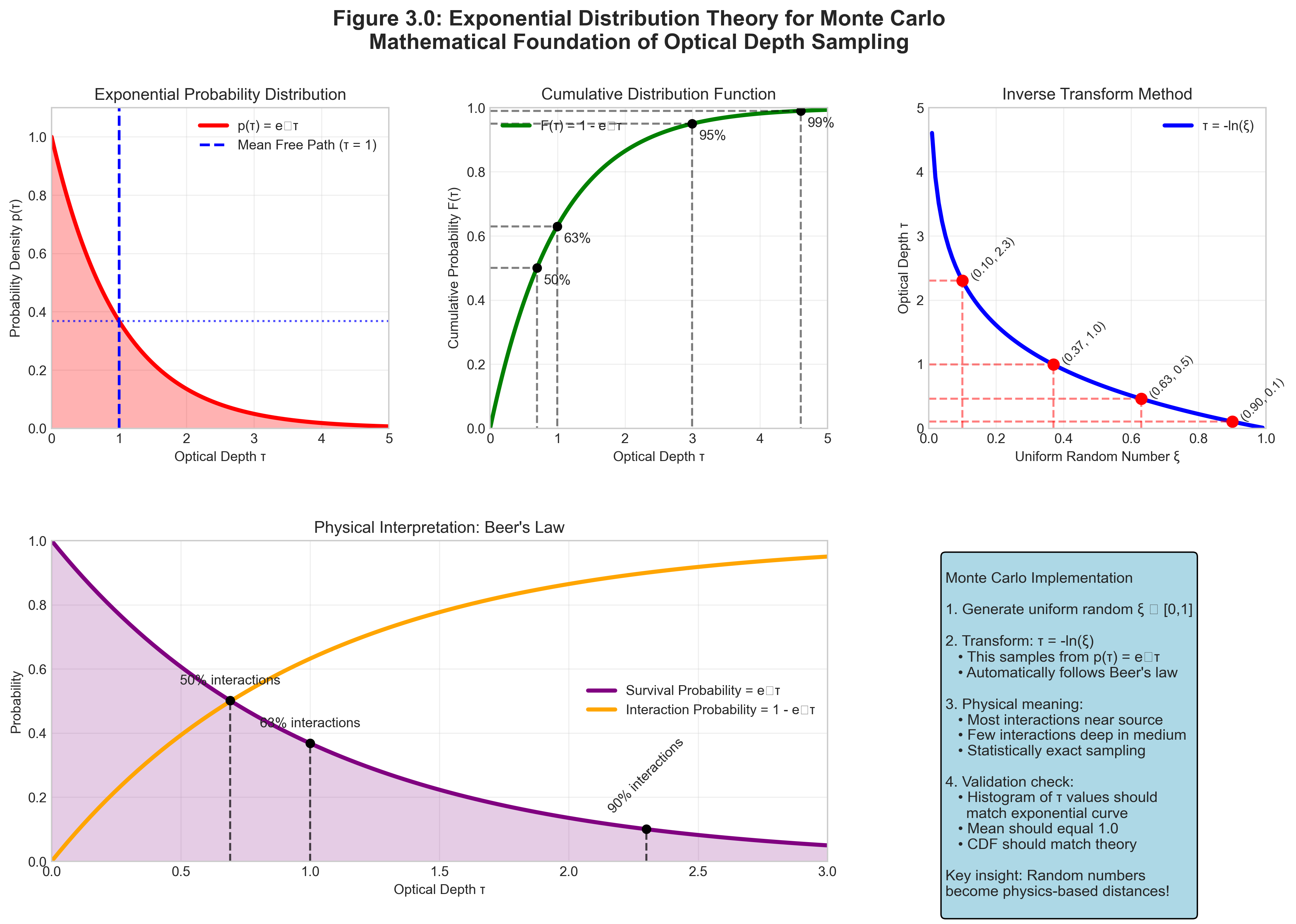
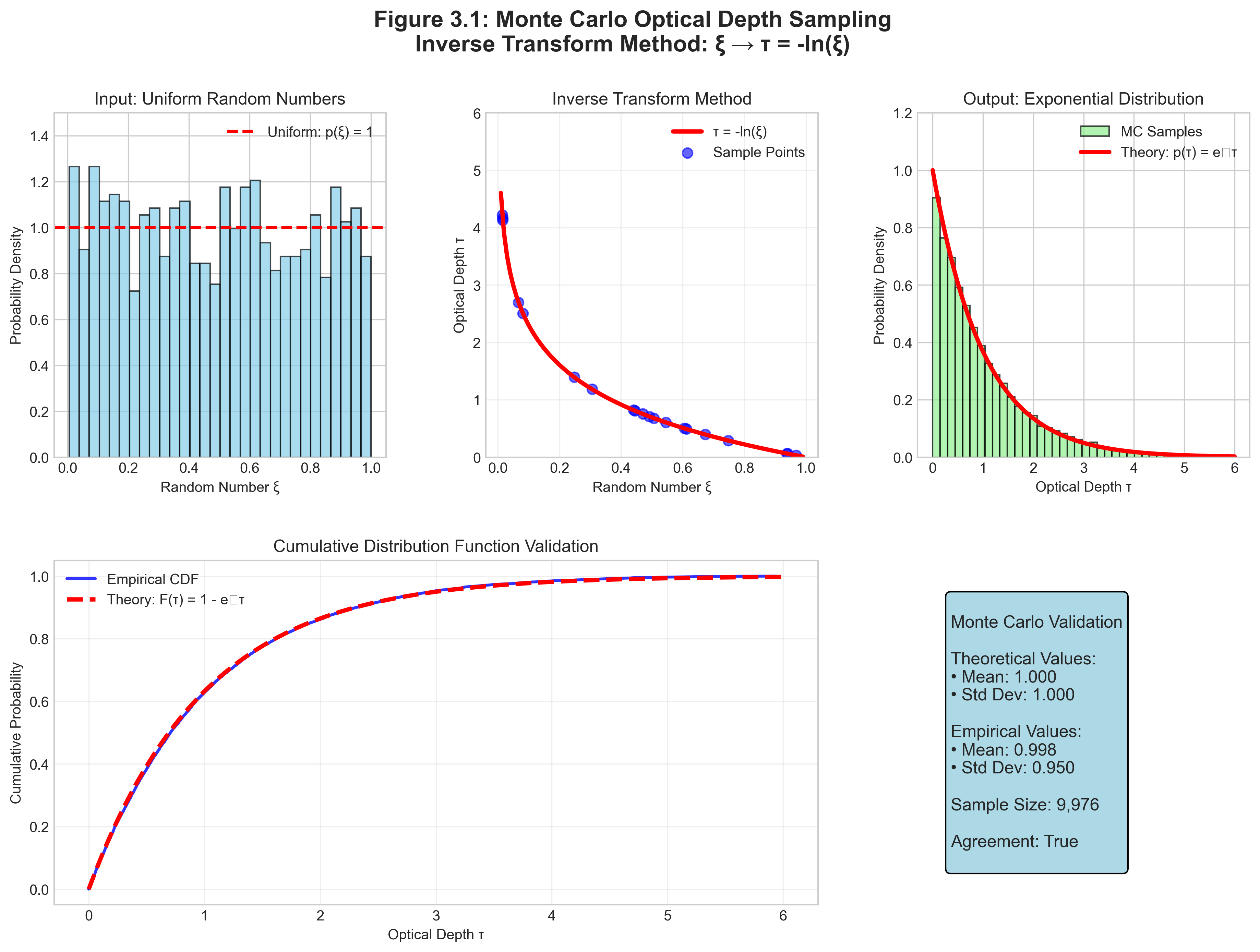
**The exponential distribution governs photon survival.** The survival probability $P(\tau) = e^{-\tau}$ (blue curve) drops to $1/e \approx 37\%$ at $\tau = 1$ and falls below 1% by $\tau \approx 5$. The interaction probability density $p(\tau) = e^{-\tau}$ (orange curve) peaks at $\tau = 0$ — most photons interact within the first mean free path. This distribution is the statistical foundation of Monte Carlo radiative transfer.

🔬 Deriving the Sampling Formula: $\tau = -\ln(\xi)$

We need to sample optical depths from the exponential distribution $p(\tau) = e^{-\tau}$. We’ll use the inverse transform method.

Step 1: Compute the cumulative distribution function (CDF)

\[F(\tau) = \int_0^\tau p(\tau') d\tau' = \int_0^\tau e^{-\tau'} d\tau' = 1 - e^{-\tau}\]

Step 2: Set CDF equal to uniform random number

\[F(\tau) = \xi\] \[1 - e^{-\tau} = \xi\]

Step 3: Solve for $\tau$

\[e^{-\tau} = 1 - \xi\] \[-\tau = \ln(1 - \xi)\] \[\tau = -\ln(1 - \xi)\]

Step 4: Simplification

Since $\xi$ is uniform on [0,1], so is $(1-\xi)$. Therefore:

\[\boxed{\tau = -\ln(\xi)}\]

Verification:

As $\xi \to 0$: $\tau \to \infty$ (photon travels forever)
As $\xi \to 1$: $\tau \to 0$ (immediate interaction)
For $\xi = e^{-1} \approx 0.368$: $\tau = 1$ (one mean free path)

Important Note: This derivation assumes we’re sampling the first interaction optical depth. In a non-uniform grid, the sampled $\tau$ is universal; the physical distance you travel before hitting that optical depth depends on the density and opacity structure you march through. For later scattering extensions, each new interaction would sample a fresh optical depth from the same distribution.

This formula is the cornerstone of Monte Carlo radiative transfer!

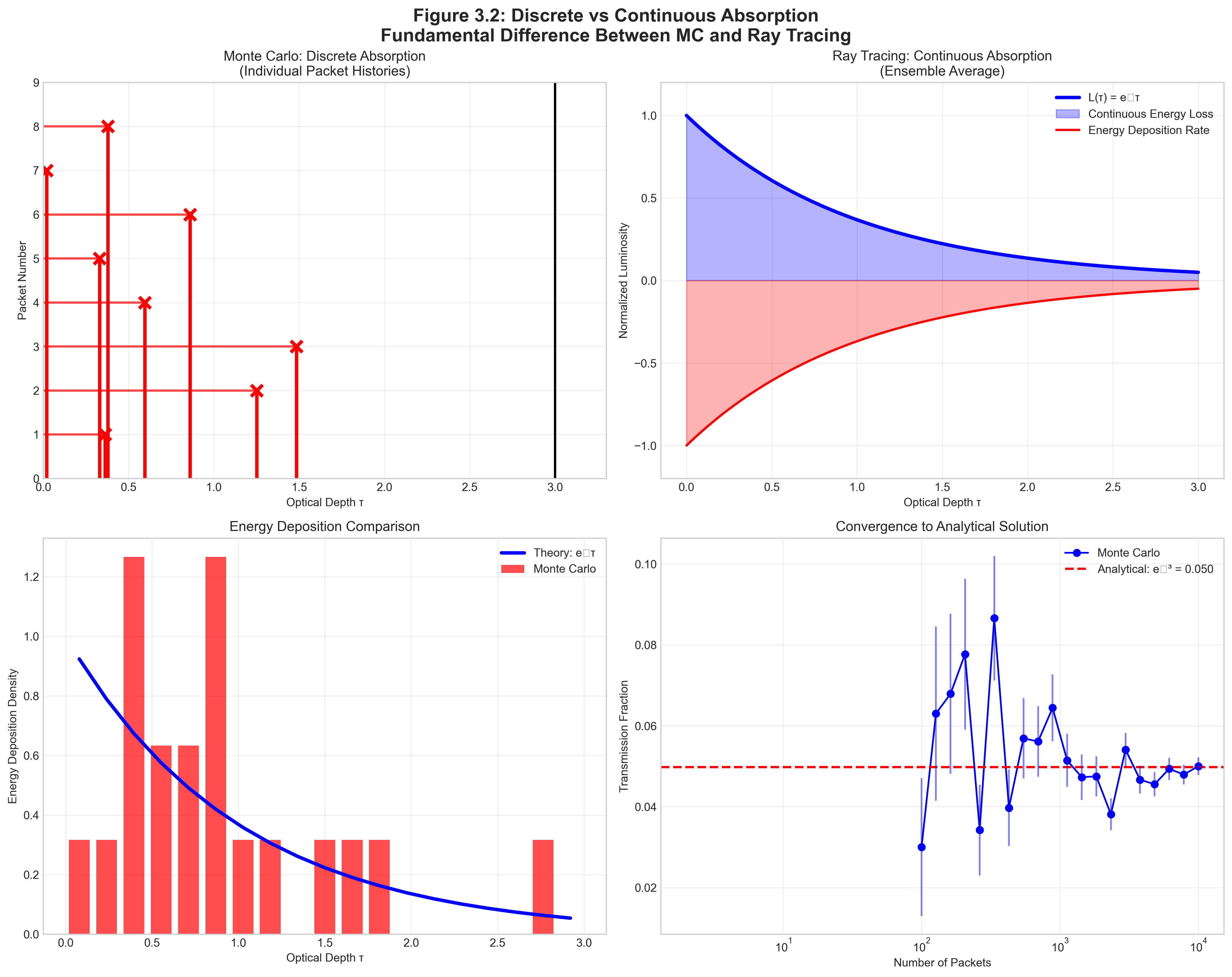
**Optical depth sampling in action.** *Left*: Histogram of $10^5$ sampled optical depths from $\tau = -\ln(\xi)$ compared to the theoretical exponential PDF $p(\tau) = e^{-\tau}$. The agreement shows that inverse transform sampling targets the correct distribution. *Right*: The CDF $F(\tau) = 1 - e^{-\tau}$ shows the probability of interaction within optical depth $\tau$, with the median interaction distance at $\tau \approx 0.69$.

3.2.2 Discrete vs. Continuous Absorption

A critical distinction that often confuses students:

For Project 3, keep the terminology sharp:

Absorption-only transport means the packet either escapes intact or deposits its full luminosity at one sampled interaction point.
In broader astrophysical language, extinction often means absorption plus scattering together.
That broader language is useful context, but it is not the bookkeeping you code first in this assignment.

Discrete Absorption (Monte Carlo - Project 3):

Packet travels WITHOUT energy loss until $\tau = \tau_{\text{target}}$
At that point, ALL energy is deposited
This is a sampling of one possible photon history

Continuous Absorption (Ray Tracing):

Packet continuously loses energy: $L(s) = L_0 e^{-\tau(s)}$
Energy is deposited gradually along the path
This computes the ensemble average directly

⚠️ Common Pitfall: Mixing Discrete and Continuous

Wrong: Reducing packet luminosity as it travels AND using discrete absorption. The issue isn’t double-counting but rather inconsistent physics — you can’t both continuously attenuate AND use discrete absorption.

# INCORRECT - Don't do this!
while traveling:
    L_packet *= exp(-tau_cell)  # Wrong for Monte Carlo!
    if tau_total >= tau_target:
        deposit_energy(L_packet)  # Inconsistent physics!

Right: Choose ONE approach

# CORRECT - Monte Carlo with discrete absorption
while traveling:
    # Packet luminosity stays constant!
    if tau_total >= tau_target:
        deposit_energy(L_packet)  # All energy here
        break

Mixing both methods violates the underlying physics of Monte Carlo sampling.

**Discrete vs. continuous absorption compared.** *Top left*: In discrete absorption (Monte Carlo), the photon packet carries full luminosity until it reaches $\tau_\text{target}$, where all energy is deposited at once. *Top right*: The net luminosity change per cell shows energy conservation — the total deposited equals the input luminosity. *Bottom left*: In continuous absorption (ray tracing), luminosity decreases exponentially along the path via $L(s) = L_0 e^{-\tau(s)}$. *Bottom right*: Both methods converge to identical results in the limit of many packets, but they must never be mixed in a single implementation.

3.2.3 Ray Marching Through Non-Uniform Media

Real media aren’t uniform. Dust density can vary, and in multi-band work the effective absorption opacity can depend on which star and band produced the packet. How do we accumulate optical depth through such media?

🔋 Algorithm: Optical Depth Integration Along a Ray

Given: Ray from position $\vec{r}_0$ in direction $\hat{n}$

Goal: Find where $\tau_{\text{accumulated}} = \tau_{\text{target}}$

Initialize
- Set $\tau_{\text{accumulated}} = 0$
- Set current position $\vec{r} = \vec{r}_0$
March through cells
- WHILE $\tau_{\text{accumulated}} < \tau_{\text{target}}$:
  - Identify current cell from position
  - Get local properties: $\rho_{\text{dust}}$, $\kappa_{\mathrm{abs}}$
  - Find distance to cell boundary: $\Delta s$
  - Calculate cell optical depth: $\Delta\tau = \kappa_\mathrm{abs} \rho_{\text{dust}} \Delta s$
  - IF $\tau_{\text{accumulated}} + \Delta\tau \geq \tau_{\text{target}}$:
    - Interaction occurs within this cell
    - Find exact position: fraction = $(\tau_{\text{target}} - \tau_{\text{accumulated}})/\Delta\tau$
    - Interaction position: $\vec{r}_{\text{int}} = \vec{r} + \text{fraction} \times \Delta s \times \hat{n}$
    - BREAK
  - ELSE:
    - Add to accumulated: $\tau_{\text{accumulated}} += \Delta\tau$
    - Move to next cell: $\vec{r} += \Delta s \times \hat{n}$
    - Check if escaped domain
Return interaction position or escape flag

This algorithm naturally handles arbitrary density distributions — the same approach works for uniform clouds, power-law profiles, or turbulent density fields. In Project 3 Phase 1A, it collapses to the cleanest possible debugging case because both $\rho_\mathrm{dust}$ and $\kappa_\mathrm{abs}$ are constant.

Ray-marching bugs that are worth fearing

These are not rare edge cases. They are the bugs most likely to consume your week:

If one direction component is zero, do not divide by it. Treat the distance to that boundary as $\infty$ in that coordinate.
If a packet lands exactly on a boundary, floating-point equality can leave it in the same cell forever. After crossing a face, nudge it a tiny distance $\epsilon \hat{n}$ into the next cell.
Boundary indexing is easy to get wrong by one cell. Always check whether your position-to-index map matches the same half-open interval convention everywhere in your code.
Use dust density, not gas density, inside $\Delta \tau = \kappa_\mathrm{abs} \rho_\mathrm{dust} \Delta s$.
Choose one absorption formalism and stay loyal to it. For Project 3 that means discrete absorption, not continuous attenuation mixed with sampled absorption events.

🔭 NGC 3603 Reality Check: Non-Uniform Dust

Real star-forming regions like NGC 3603 don’t have uniform dust. The density might follow:

\[\rho_{\text{dust}}(r) = \rho_0 \left(1 + \frac{r^2}{r_c^2}\right)^{-1}\]

where $r_c \sim 0.1$ pc is the core radius.

Optical depth to the center: \[\tau = \int_0^R \kappa \rho_0 \left(1 + \frac{r^2}{r_c^2}\right)^{-1} dr = \kappa \rho_0 r_c \arctan(R/r_c)\]

For $R \gg r_c$: $\tau \approx \kappa \rho_0 r_c \times \pi/2$

Key insight: The optical depth converges! Even infinite clouds have finite optical depth if density drops fast enough. This is why we can see through galaxy halos — density drops faster than radius increases.

3.2.4 Worked Hand-Trace: One Packet from Emission to Absorption

Before you code, it helps to watch one packet live its whole life.

Let’s use a hand-trace variant of the Project 3 Phase 1A setup:

one star at the box center,
V-band only,
uniform dust density $\rho_\mathrm{dust} = 3.84 \times 10^{-23}~\mathrm{g\,cm^{-3}}$,
constant absorption opacity $\kappa_V = 7300~\mathrm{cm^2\,g^{-1}}$,
a $17^3$ debugging grid inside a box of side length $L = 1~\mathrm{pc}$.

We choose an odd grid here on purpose. A $17^3$ grid has a true central cell, so the source can sit at the center of that cell without living exactly on a grid boundary. That avoids teaching an indexing pathology in the very example students are most likely to copy while debugging.

The cell width is

\[\Delta x = \frac{L}{17} \approx 0.0588~\mathrm{pc} = 1.82 \times 10^{17}~\mathrm{cm}.\]

Suppose this packet history unfolds:

Source selection: there is only one star, so that star emits the packet.
Emission position: the packet starts at the center of the central cell, so the first step to a boundary is half a cell.
Direction sampling: we sample an isotropic direction and happen to get $\hat{n} = (1, 0, 0)$.
Interaction optical depth: draw $\xi = 0.86$, so

\[\tau_{\text{target}} = -\ln(0.86) = 0.151.\]
Ray marching through cells:

The optical depth across one full cell is

\[\Delta \tau_{\text{cell}} = \kappa_V \rho_\mathrm{dust} \Delta x = 7300 \times 3.84 \times 10^{-23} \times 1.82 \times 10^{17} \approx 0.051.\]

Because the source begins at the middle of the central cell, the first step is only half a cell:

\[\Delta \tau_{\text{half-cell}} \approx 0.025.\]
- After the first half-cell crossing: $\tau_{\text{accumulated}} = 0.025$
- After the next full cell: $\tau_{\text{accumulated}} = 0.076$
- After the next full cell: $\tau_{\text{accumulated}} = 0.127$
- The packet still has not interacted, so it enters the next cell.
Interaction inside the next cell:

The remaining optical depth is

\[\tau_{\text{remain}} = 0.151 - 0.127 = 0.024.\]

So the packet travels a fraction

\[f = \frac{\tau_{\text{remain}}}{\Delta \tau_{\text{cell}}} \approx \frac{0.024}{0.051} \approx 0.47\]

of that cell before absorption.

That puts the interaction point at about

\[x \approx \left(2.5 + 0.47\right)\Delta x \approx 0.175~\mathrm{pc}, \qquad y = 0, \qquad z = 0.\]
Bookkeeping:
- The packet does not contribute to $L_\mathrm{esc}$.
- Its full luminosity $L_\mathrm{packet}$ is added to the absorption tally in that cell.
- Energy conservation bookkeeping updates:
  
  \[L_\mathrm{abs} \leftarrow L_\mathrm{abs} + L_\mathrm{packet}.\]

That is the whole logic of discrete absorption in miniature: sample $\tau_{\text{target}}$, accumulate optical depth cell by cell, stop when you hit it, then deposit the packet’s full luminosity once. The implementation lesson is as important as the physics lesson: be explicit about where the source sits relative to cell boundaries, or your first debugging example can be ambiguous before your code even starts.

3.2.5 Statistical Validation

How do we know our Monte Carlo code is correct? Statistical tests!

🔬 Validation Unit Test: Uniform Slab

Setup: Uniform slab with total optical depth $\tau_0$

Analytical solution: Transmission = $e^{-\tau_0}$

Monte Carlo test — samples n_packets through a slab of optical depth tau_0, returns escape fraction with Poisson error for comparison against $e^{-\tau_0}$:

def test_uniform_slab(tau_0, n_packets=10000):
    escaped = 0
    for i in range(n_packets):
        tau_target = -log(random())
        if tau_target > tau_0:
            escaped += 1
    
    f_escape_mc = escaped / n_packets
    f_escape_analytical = exp(-tau_0)
    
    # Statistical error (Poisson)
    sigma = sqrt(f_escape_mc * (1 - f_escape_mc) / n_packets)
    
    # Check agreement within 3-sigma
    deviation = abs(f_escape_mc - f_escape_analytical) / sigma
    assert deviation < 3.0, f"Failed: {deviation:.1f} sigma deviation"
    
    return f_escape_mc, sigma

Results for $\tau_0 = 2.0$:

Analytical: $e^{-2} = 0.1353$
Monte Carlo (N=10⁴): $0.136 \pm 0.003$ ✓
Monte Carlo (N=10⁶): $0.1354 \pm 0.0003$ ✓

The standard error scales as $N^{-1/2}$ as predicted, while the variance scales as $N^{-1}$.

This slab problem is a great unit test because it isolates the exponential sampling logic cleanly. But it is not the same geometry as Project 3 Phase 1A.

Project 3 validation is centered-star-in-cube, not slab transmission

For Project 3 Phase 1A, the required validation case is a single centered star in a uniform cube. In that geometry, the packet path length depends on direction:

The shortest escape path is face-normal, with distance $L/2$.
The longest escape path is toward a corner, with distance $L\sqrt{3}/2$.

That immediately gives analytic bounds on the Monte Carlo escape fraction:

\[ \exp\!\left(-\kappa \rho \frac{L\sqrt{3}}{2}\right) \;<\; f_\mathrm{esc}^\mathrm{MC} \;<\; \exp\!\left(-\kappa \rho \frac{L}{2}\right). \]

Why are these bounds sensible?

The face-normal path is the upper bound because it is the shortest possible route out of the cube, so it gives the largest escape probability.
The corner path is the lower bound because it is the longest possible route out of the cube, so it gives the smallest escape probability.

So keep both ideas in your toolbox:

The slab test checks whether your exponential sampling logic is sane.
The centered-cube bounds check whether your actual Project 3 geometry and ray marching are sane.
Energy conservation and $N^{-1/2}$ convergence check whether the full Monte Carlo estimator is behaving statistically the way it should.

Validation Ladder: Build Trust One Layer at a Time

Test	What it checks	What kind of bug it catches
Inverse-transform histogram for $\tau = -\ln(\xi)$	Your random sampling matches the target exponential distribution	Broken RNG usage, wrong sign in the logarithm, malformed sampler
Uniform slab transmission	The survival/escape logic matches $e^{-\tau}$ in the simplest geometry	Confusing survival probability with interaction probability
Centered-cube analytic bounds	Your actual Project 3 geometry and ray marching behave sensibly	Wrong path lengths, wrong boundary handling, wrong cell traversal
Energy conservation	Every packet ends up either escaped or absorbed	Lost packets, dropped luminosity, inconsistent bookkeeping
$N^{-1/2}$ standard-error scaling	The Monte Carlo estimator behaves statistically as expected	Hidden systematics masquerading as noise, incorrect uncertainty estimates

3.3 Practical Implementation Strategies

Priority: 🟡 Important.

Moving from algorithm to efficient code requires careful attention to computational strategies. Here we focus on the implementation choices that matter most for Project 3 first, then keep a few richer MCRT ideas on the table as optional extensions.

3.3.1 What Changes, and What Does Not, Across Project 3

The most important implementation idea in this whole reading is that the core transport loop stays stable across the project.

Phase ladder: one transport loop, changing configuration

Phase 1A: One centered star, V-band only, constant-opacity debugging case

You debug the core loop: emit packet, sample $\tau_{\text{target}}$, ray march, absorb or escape, update bookkeeping.
Validation is front and center: centered-cube bounds, energy conservation, and $N^{-1/2}$ convergence.

Phase 1B: All 5 stars, still V-band only

The transport loop does not change.
The only new idea is source selection: emit packets from stars with probabilities proportional to their V-band luminosities.

Phase 2: B, V, K bands

The transport loop still does not change.
The new work is opacity and luminosity bookkeeping: each star now has a different band luminosity and a different effective band opacity.

If you find yourself rewriting propagate_packet() between phases, that is a warning sign. The whole point of the project design is that the algorithm stabilizes early, and later phases mostly change inputs and bookkeeping.

Mini software architecture sketch

One clean way to keep the codebase disciplined is to separate sampling, transport, and bookkeeping:

sample_source(...)
sample_direction(...)
sample_tau(...)
locate_cell(...)
advance_to_boundary(...)
propagate_packet(...)
record_escape(...)
record_absorption(...)

The design principle is simple:

propagate_packet(...) should remain stable across Phase 1A, 1B, and 2.
Phase 1B should mostly change sample_source(...).
Phase 2 should mostly change opacity lookup and luminosity bookkeeping.

That is how you avoid turning one elegant transport algorithm into three slightly different, slightly broken ones.

Pre-Flight Sanity Check: Mean Free Path Before You Code

Before you write a line of transport code, estimate two scales:

\[\ell = \frac{1}{\kappa_\mathrm{abs} \rho_\mathrm{dust}}, \qquad \tau_\mathrm{box} \sim \kappa_\mathrm{abs} \rho_\mathrm{dust} L. \]

For the Project 3 Phase 1A debugging values,

\[\kappa_\mathrm{abs} \rho_\mathrm{dust} \approx 2.8 \times 10^{-19}~\mathrm{cm^{-1}},\]

\[\ell \approx 3.6 \times 10^{18}~\mathrm{cm} \approx 1.16~\mathrm{pc}, \qquad \tau_\mathrm{box} \sim 0.87.\]

That already tells you what “reasonable” should look like:

If $\ell \gg L$, most packets should escape.
If $\ell \ll L$, most packets should be absorbed.
If $\tau_\mathrm{box} \sim 1$, both escape and absorption should occur appreciably.

This back-of-the-envelope check catches the failures that waste the most time:

wrong units,
dust-versus-gas density confusion,
absurd opacity values,
“all packets escape” or “nothing escapes” behavior that is obvious before you even profile the code.

Deterministic Debug Mode

Before debugging one million packets, debug one packet.

Create a mode where you:

fix the RNG seed,
emit exactly one packet,
optionally hard-code the direction and $\xi$,
print every crossed cell,
print $\Delta s$, $\Delta \tau$, and $\tau_\mathrm{accumulated}$ at each step,
confirm whether the packet escapes or absorbs,
compare the output against your hand trace.

This turns Monte Carlo from random soup into an inspectable algorithm. It is one of the fastest ways to find boundary bugs, indexing mistakes, and unit errors.

🔧 When Your Monte Carlo Code Fails

Diagnostic Workflow - Check in This Order:

All packets escape?
- Check opacity units (dust vs. gas density)
- Verify κ values are ~10⁴ cm²/g for dust, not ~10⁻¹ cm²/g for gas
- Check if you’re using mass or number density
No packets escape?
- Verify τ sampling: should use tau = -log(random()), not log(random())
- Check for infinite loops in ray marching
- Ensure boundary conditions are implemented
Results don’t converge?
- Check random number generator quality (avoid rand(), use Mersenne Twister)
- Verify sufficient packets: need ~100 per optically thin region
- Check for systematic errors in path length calculation
Energy not conserved?
- Look for boundary condition bugs (packets lost at edges)
- Check floating-point precision in optical depth accumulation
- Verify all interaction types are handled
Noisy spatial maps?
- Increase packet count before reaching for advanced variance reduction
- Check that energy deposition is correctly binned
- Then consider optional variance-reduction ideas if needed
Wrong escape fraction?
- Ensure using ONE method consistently (discrete OR continuous)
- Validate against the centered-cube bounds first
- Check wavelength-dependent opacity implementation

⚡ Performance Profiling Your Monte Carlo Code

Why Profile? Understanding where your code spends time is essential for optimization. Most Monte Carlo codes have predictable bottlenecks.

When to Profile: - Code runs slower than expected (< 10³ packets/second) - Need to scale to large simulations (> 10⁶ packets) - Comparing different algorithmic approaches - Before implementing parallelization

How to Profile in Python:

import cProfile
import pstats
import time

def profile_monte_carlo():
    # Create profiler
    profiler = cProfile.Profile()
    profiler.enable()
    
    # Your Monte Carlo simulation here
    escape_fraction = run_simulation(n_packets=10000)
    
    profiler.disable()
    
    # Analyze results
    stats = pstats.Stats(profiler)
    stats.sort_stats('cumulative')
    stats.print_stats(10)  # Top 10 functions
    
    return escape_fraction

# Alternative: line-by-line profiling
%load_ext line_profiler
%lprun -f your_main_function your_main_function()

Common Bottlenecks (in order of frequency): 1. Ray-cell intersection calculations (~40% of time) - Solution: Pre-compute grid boundaries, use efficient data structures 2. Random number generation (~20% of time)
- Solution: Vectorize RNG calls, use quality generators 3. Optical depth accumulation (~15% of time) - Solution: Use efficient path integration, avoid repeated calculations 4. Grid boundary checks (~10% of time) - Solution: Smart grid traversal algorithms

Structured-grid insight: If your grid is Cartesian, you do not have to recompute geometry from scratch in every cell forever. Naive per-cell boundary finding is perfectly fine for a first correct implementation, but structured grids admit faster voxel-traversal or DDA-style stepping. In practice, ray-cell intersection logic is often a more important optimization target than shaving a few nanoseconds off random-number calls.

Optimization Strategy:

# Before optimization - measure baseline
start = time.time()
result = run_simulation(1000)
baseline_time = time.time() - start
print(f"Baseline: {1000/baseline_time:.0f} packets/second")

# After optimization - measure improvement
start = time.time()
result_optimized = run_simulation_optimized(1000)
optimized_time = time.time() - start
speedup = baseline_time / optimized_time
print(f"Optimized: {1000/optimized_time:.0f} packets/second")
print(f"Speedup: {speedup:.1f}x")

Performance Targets: - Simple uniform medium: ~10⁵ packets/second (Python) - 3D grid (100³): ~10⁴ packets/second
- With scattering: ~10³ packets/second - Production codes (C/Fortran): 10-100$\times$ faster

3.3.2 Luminosity Weighting for Multiple Sources

When you have multiple sources with different luminosities, how do you ensure proper sampling?

🔋 Algorithm: Luminosity-Weighted Source Selection

Given: N stars with luminosities $L_1, L_2, ..., L_N$

Goal: Select sources proportional to their contribution

Precompute cumulative distribution

L_total = sum(L_i)
CDF[0] = 0
for i = 1 to N:
    CDF[i] = CDF[i-1] + L_i/L_total

For each packet:
- Draw random number $\xi \in [0,1]$
- Binary search to find i where: CDF[i-1] $\le$ ξ < CDF[i]
- Emit from source i
- Packet carries luminosity: $L_{\text{packet}} = L_{\text{total}}/N_{\text{packets}}$

Key: All packets carry equal luminosity, but more packets come from brighter sources.

💭 Think About It: Why Equal-Weight Packets?

Question: Why not give each star a fixed number of packets with different weights?

Answer: Equal-weight packets have several advantages:

Simpler statistics: Each packet contributes equally to uncertainties
Better sampling: Bright sources automatically get more packets
Easier parallelization: Any processor can handle any packet
Adaptive refinement: Can add more packets without reweighting

The alternative (weighted packets) is useful for variance reduction but complicates error analysis.

3.3.3 Optional Extensions: Variance Reduction Beyond the Core Project

Standard Monte Carlo converges slowly ($\sigma \propto N^{-1/2}$). Variance reduction speeds convergence without bias, but these techniques are not required for the core Project 3 transport algorithm. They belong to the “what comes next?” category once your absorption-only code is correct and validated.

🔧 Technique: Forced First Interaction

For optically thick media where most photons interact quickly, force the first interaction:

Standard approach: Many packets absorbed near source, few reach interesting regions

Forced first interaction:

First interaction always occurs (no escape on first segment)
Sample position from: $p(\tau) = e^{-\tau}/(1 - e^{-\tau_{\text{max}}})$
Weight packet by probability it would have escaped: $w = e^{-\tau_{\text{max}}}$

Result: Better sampling of full domain with same number of packets

🔧 Technique: Russian Roulette

When packets become very weak (after many scatterings), terminate probabilistically:

def russian_roulette(packet, threshold=0.01):
    if packet.luminosity < threshold * packet.initial_luminosity:
        p_survive = packet.luminosity / (threshold * packet.initial_luminosity)
        if random() < p_survive:
            # If packet survives with probability p, its weight must increase by 1/p
            # to maintain average energy conservation
            packet.luminosity /= p_survive
            return 'continue'
        else:
            return 'terminate'
    return 'continue'

Conservation: On average, the same energy is tracked, but with fewer packets.

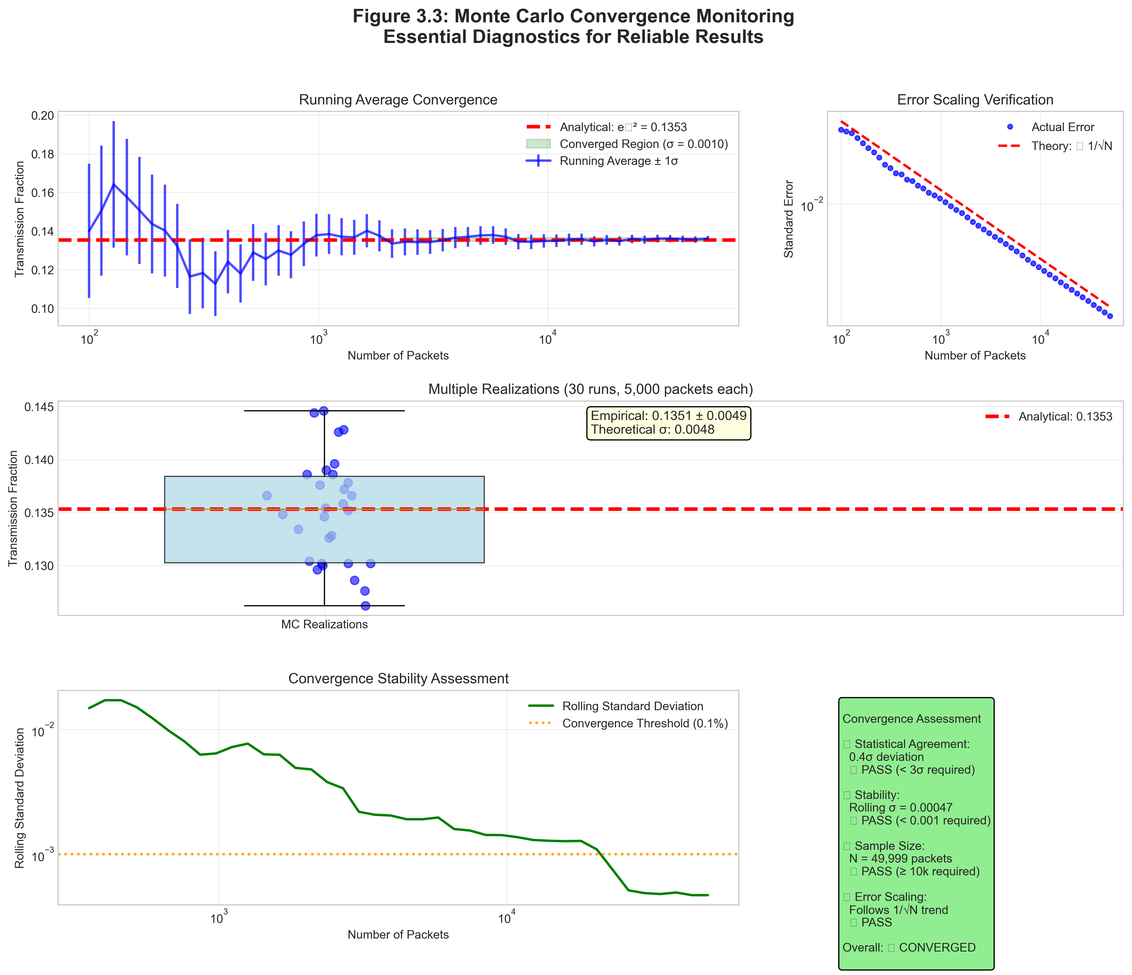
3.3.4 Convergence Monitoring

How many packets are enough? Monitor convergence!

📊 Convergence Diagnostics

1. Running mean and standard error:

def monitor_convergence(results, n_checkpoints=10):
    checkpoint_size = len(results) // n_checkpoints
    means = []
    errors = []
    
    for i in range(1, n_checkpoints + 1):
        sample = results[:i * checkpoint_size]
        means.append(mean(sample))
        errors.append(std(sample) / sqrt(len(sample)))
    
    # Plot means with error bars
    # Should see convergence to stable value

2. Variance scaling test:

# Run with N = 10^3, 10^4, 10^5, 10^6
# Plot log(error) vs log(N)
# Slope should be -0.5

3. Spatial convergence:

Check that all regions have sufficient packets
Energy deposition should be smooth, not noisy
Increase N if some cells have < 100 packets

4. Convergence Criteria for Project 3:

Energy conservation: Check that $L_\mathrm{in} = L_\mathrm{abs} + L_\mathrm{esc}$ to your stated tolerance
Cube-bound validation: In Phase 1A, verify that $f_\mathrm{esc}$ lies between the centered-cube analytic bounds
Error Scaling: Standard error should decrease as $N^{-1/2}$, while the variance decreases as $N^{-1}$
Stability: Running averages should settle rather than drift systematically as you add packets

Rare-event caution

When $f_\mathrm{esc}$ is very small, remember that the estimator is fundamentally binomial. If only a handful of packets escape, naive normal-approximation intuition can get shaky. In that regime, ask whether your uncertainty estimate is really being driven by only a few escape events.

**Convergence monitoring for Monte Carlo radiative transfer.** *Left*: The running average of the escape fraction converges toward the analytical value (dashed line) as the number of packets increases. The shaded region shows the $\pm 1\sigma$ confidence interval, whose standard-error width narrows as $N^{-1/2}$ while the variance falls as $N^{-1}$. *Right*: Log-log plot confirming that the standard error scales as $N^{-1/2}$ (solid line follows the theoretical slope). Use both diagnostics — a stable running average AND the expected error scaling — to verify convergence in your Project 3 implementation.

3.3.5 Multi-Wavelength Implementation

For problems with wavelength-dependent opacity (like Project 3):

From $\kappa_\lambda$ to band-averaged opacity

The Draine table gives you a wavelength-dependent absorption opacity $\kappa_\lambda$. Your transport code, however, needs a practical opacity value for a packet in a specific photometric band.

That is why Project 3 asks for an effective band opacity:

\[ \langle\kappa\rangle_{\mathrm{band,star}} = \frac{\int_{\lambda_1}^{\lambda_2} \kappa_\lambda B_\lambda(T_{\mathrm{eff,star}})\, d\lambda} {\int_{\lambda_1}^{\lambda_2} B_\lambda(T_{\mathrm{eff,star}})\, d\lambda}. \]

Read this formula physically:

$\kappa_\lambda$ tells you what the dust does as a function of wavelength.
$B_\lambda(T_{\mathrm{eff,star}})$ tells you how strongly a given star emits at each wavelength.
The ratio produces the effective opacity seen by photons from that star in that band.

This means a hot O star and a cooler A star can have different effective opacities in the same nominal V band. They are moving through the same dust, but they weight the wavelength-dependent dust curve differently across the bandpass.

That is the Project 3 interpretation to carry into Phase 2: the transport loop is unchanged, but the opacity lookup becomes star-dependent and band-dependent.

🔋 Algorithm: Multi-Band Monte Carlo

Project 3 recommendation: separate runs per band.

for band in ["B", "V", "K"]:
    L_band_total = sum(star.L_band[band] for star in stars)
    for packet in range(N):
        star = sample_source(weighted by star.L_band[band])
        kappa_abs = star.kappa_band[band]
        propagate_packet(star, band, kappa_abs)
    escape_fraction[band] = L_escaped[band] / L_band_total

Pros: Clean statistics per band, straightforward debugging, matches the project phase structure
Cons: 3$\times$ the transport runs

More advanced alternative: one mixed run that samples bands directly.

total_luminosity = sum over bands and stars
for packet in range(N):
    band = sample_band(weighted by luminosity)
    star = sample_source(weighted within that band)
    kappa_abs = opacity_table[star, band]
    propagate_packet(star, band, kappa_abs)

Pros: One run, automatic importance sampling
Cons: Uneven statistics across bands
Not recommended for the first implementation of Project 3

Recommendation: For Project 3, use the first approach. It keeps the bookkeeping transparent and reinforces the main conceptual lesson: same transport loop, different band-specific inputs.

3.3.6 Common Implementation Pitfalls

⚠️ Implementation Pitfalls to Avoid

1. Random Number Generator Quality:

✗ Using poor RNG (e.g., simple linear congruential)
✅ Use Mersenne Twister or PCG
Test: Consecutive pairs shouldn’t correlate

2. Boundary Condition Bugs:

✗ Packets stuck on boundaries due to floating-point
✅ Add small epsilon when crossing boundaries
Test: No packets should make > 1000 cell crossings

3. Cell-Indexing Bugs:

✗ Using inconsistent rules for which cell owns a boundary point
✅ Adopt one half-open interval convention and test boundary cases explicitly
Test: Hand-trace a packet that crosses a face exactly

4. Dust vs. Gas Density Confusion:

✗ Using $\rho_\mathrm{gas}$ inside $\Delta \tau = \kappa \rho \Delta s$
✅ Convert once to $\rho_\mathrm{dust}$ and use that consistently in transport
Test: Check whether your optical depths are larger than expected by a factor of 100

5. Memory Management:

✗ Storing all packet histories (memory explosion)
✅ Process packets one at a time or in batches
Only store final results and statistics

6. Numerical Precision:

✗ Using float32 for optical depth accumulation
✅ Use float64 for τ (accumulation errors matter)
Test: Results shouldn’t depend on path subdivision

7. Absorption Formalism Drift:

✗ Continuously attenuating packet luminosity and also triggering discrete absorption
✅ Keep packet luminosity constant until a sampled absorption event or escape
Test: Audit one packet history by hand and confirm it deposits all or nothing

8. Energy Conservation:

✗ Losing energy at boundaries or in scattering
✅ Track total energy budget:

assert abs(E_in - E_out - E_absorbed) / E_in < 1e-10

💻 Computational Cost Analysis

Based on empirical benchmarks for Python/NumPy implementations:

Scenario	Packets/sec*	Time for 10⁶ packets	Memory**	Key Bottleneck
Uniform medium	~10⁵-10⁶	1-10 seconds	~10 MB	RNG & math ops
3D grid (128³)	~10⁴-10⁵	20s-2 min	~100 MB	Ray-cell intersections
+ Scattering (ω=0.6)	~10³-10⁴	2-20 min	~100 MB	Multiple interactions
+ Complex opacity	~5$$10²-5$$10³	3-30 min	~500 MB	Table lookups
High resolution (528³)	~10²-10³	20 min-3 hrs	~4 GB	Memory access

Single-core performance on modern CPU (2020+). Actual speeds vary with:

Implementation quality (vectorization, caching)
Specific geometry and optical depths
Output requirements (binning resolution)

Memory breakdown per packet:

Position (3$$8 bytes) + Direction (3$$8 bytes) = 48 bytes
Luminosity + wavelength + auxiliary = ~32 bytes
Total: ~80-100 bytes/packet active memory

Scaling relationships:

Speed $\propto$ 1/(grid resolution) for ray marching
Speed $\propto$ 1/(1 + ⟨n_scatters⟩) for scattering
Memory $\propto$ (grid resolution)³ for field storage
Standard error $\propto N^{-1/2}$ regardless of complexity

⚠️ Important: These are order-of-magnitude estimates. Always profile your specific implementation!

🔭 NGC 3603: Computational Requirements

Let’s estimate packets needed for NGC 3603 with $A_V = 5$ mag:

Escape fraction: $f_{\text{esc}} \approx e^{-\tau_V} \approx e^{-4.6} \approx 0.01$

For 1% relative error in escape fraction: \[N \approx \frac{1 - f_{\text{esc}}}{\epsilon^2 f_{\text{esc}}} = \frac{0.99}{(0.01)^2 \times 0.01} = 10^6 \text{ packets}\]

For 3D grid with 128³ cells:

Average packets per cell: 1
Need ~100 per cell for smooth maps
Total needed: ~10⁸ packets

Computational time (order-of-magnitude estimates only):

Simple Python: ~10³ packets/second $\to$ 10³ seconds
Optimized Python (NumPy): ~10⁵ packets/second $\to$ 10 seconds
C/Fortran: ~10⁶ packets/second $\to$ 1 second
GPU parallel: ~10⁸ packets/second $\to$ 0.01 seconds

Optimization matters!

3.3.7 Connection to Statistical Foundations

🔗 Connecting to Module 1: Statistical Principles

The Monte Carlo method leverages key concepts from Module 1:

Central Limit Theorem Application:

Your escape fraction estimate $\hat{f}$ from $N$ packets has:

Mean: E[] = f_true (unbiased estimator)
Standard error: $\sigma_\hat{f} = \sqrt{(f(1-f)/N)}$
Distribution: Normal for large $N$

Confidence Intervals: For 95% confidence: $\hat{f} ± 1.96\sigma_\hat{f}$

Variance Reduction as Importance Sampling: Forcing first interactions samples from: \[p(τ) = \frac{e^{-τ}}{(1 - e^{-τ_\text{max}})}\] instead of the natural distribution, reducing variance in important regions.

Poisson Process Connection: Along path length, the interaction hazard is

\[\chi = \kappa_\mathrm{abs} \rho_\mathrm{dust}.\]

That means the natural transport variable is optical depth,

\[d\tau = \chi \, ds.\]

If you choose to parameterize motion by time for photons moving at $c$, then the corresponding interaction rate is

\[c\chi.\]

So the clean hierarchy is:

along path length, the hazard is $\chi$,
in time, the rate is $c\chi$,
in Monte Carlo transport, the sampled random variable is usually optical depth $\tau$.

3.4 Looking Ahead: Scattering Beyond Project 3

Priority: 🟡 Enrichment / future scope.

Project 3 does not require scattering in the transport loop. Still, it is worth seeing why scattering makes full radiative transfer richer and harder. Once scattering enters, packets can change direction after interactions, and the bookkeeping is no longer the clean absorption-only story you are coding first.

3.4.1 The Scattering Decision

When a photon interacts with dust, it either absorbs or scatters based on the albedo:

🔋 Algorithm: Processing Scattering Interactions

At each interaction point:

Determine interaction type

if random() < albedo:
    # Scattering
    new_direction = sample_phase_function(old_direction)
    # Packet continues with new direction
else:
    # Absorption
    deposit_energy(position, packet.luminosity)
    # Packet terminates

For isotropic scattering:
- Sample new direction uniformly on sphere
- Same as initial emission direction

For anisotropic scattering (Henyey-Greenstein):

Phase function: $p(\theta) = \frac{1-g^2}{(1+g^2-2g\cos\theta)^{3/2}}$
g = asymmetry parameter (-1: back, 0: isotropic, +1: forward)

Sampling Algorithm (Inverse Transform):

def sample_henyey_greenstein(g):
    xi = random()
    if abs(g) < 1e-3:  # Isotropic case
        cos_theta = 1 - 2*xi
    else:
        s = (1 - g*g) / (1 - g + 2*g*xi)
        cos_theta = (1 + g*g - s*s) / (2*g)

    phi = 2*pi*random()
    return angles_to_direction(cos_theta, phi)

Continue propagation
- Sample new $\tau_{\text{target}}$
- Repeat until absorbed or escaped

3.4.2 Why Scattering Increases Complexity

💭 Think About It: The Scattering Random Walk

Consider a photon in a medium with albedo $\omega = 0.9$ and optical depth $\tau = 10$.

Without scattering: Probability of escape = $e^{-10} \approx 4 \times 10^{-5}$

With scattering: The photon can scatter many times, taking a random walk. On average:

Number of scatterings before absorption: $\omega/(1-\omega) = 9$
Each scattering redirects the photon
Effective path length increases
But probability of eventual escape also increases!

Result: More photons escape, but they take longer, more complex paths. This is why Monte Carlo excels here — tracking these paths analytically would be impossible.

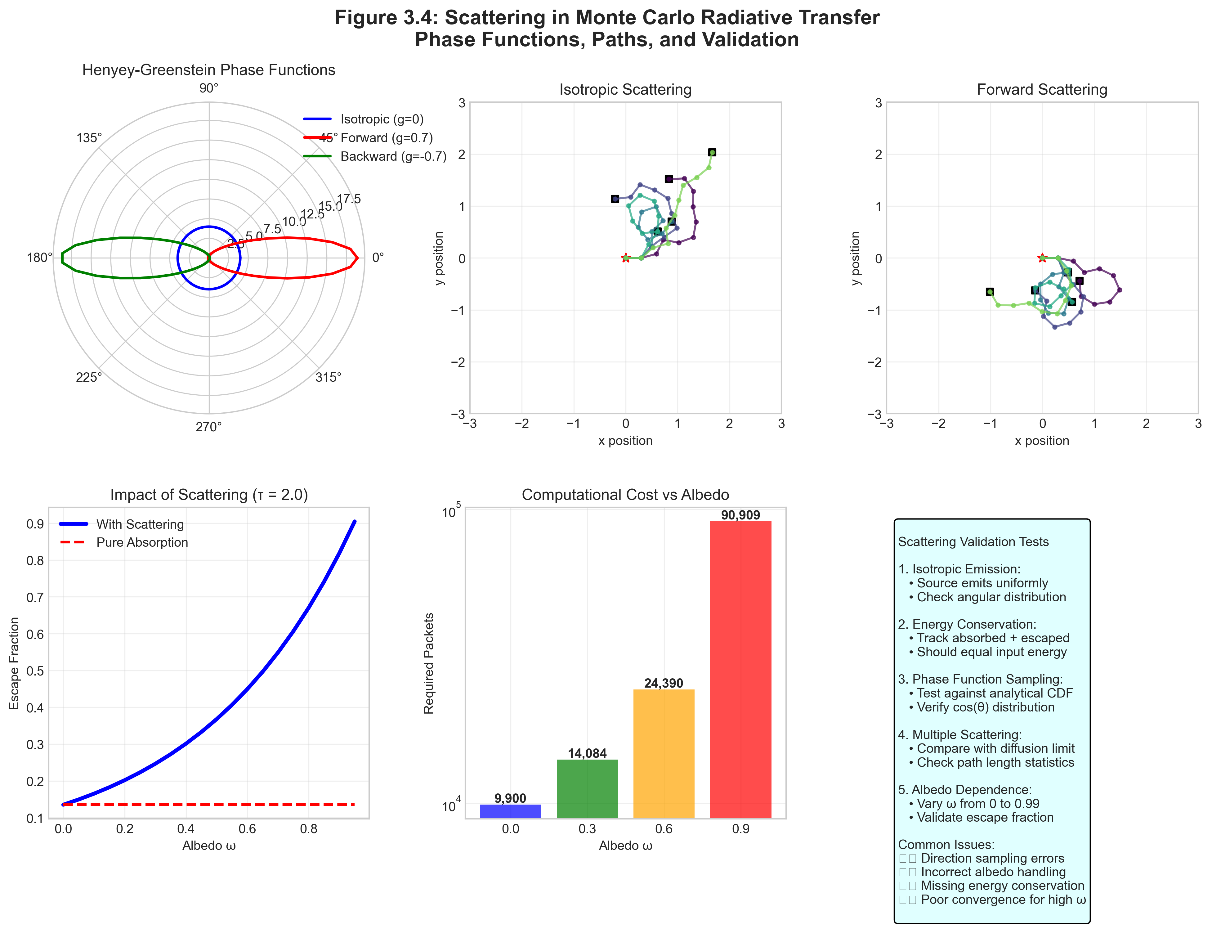
**How scattering changes photon transport.** *Left*: Without scattering ($\omega = 0$), photons travel in straight lines and are absorbed at their interaction point. *Right*: With scattering ($\omega = 0.9$), photons undergo a random walk, changing direction at each scattering event. Some photons that would have been absorbed in the pure-absorption case now escape after multiple scatterings — increasing the effective escape fraction but requiring many more packets for convergence.

3.4.3 Convergence with Scattering

Scattering slows convergence because:

Photons undergo multiple interactions
Path lengths become variable
Correlation between packets increases

📊 Convergence in Scattering Media

Empirical scaling for required packets (approximation that depends on geometry and optical depth):

Without scattering: \[N \propto \frac{1}{\epsilon^2}\]

With scattering (albedo $\omega$): \[N \propto \frac{1}{\epsilon^2} \times \frac{1}{1-\omega}\]

For $\omega = 0.6$ (typical dust), need ~2.5$\times$ more packets than pure absorption.

For $\omega = 0.9$, need ~10$\times$ more packets!

Variance reduction becomes essential for high albedo.

Warning

Verification Is Essential: Every implementation must be validated against known solutions:

Beer’s Law Test: Pure absorption must give T = e^(-τ)
Conservation Test: Energy in = Energy out + Energy absorbed (to machine precision)
Isotropy Test: Isotropic source must produce isotropic escape
Convergence Test: Standard error must scale as $N^{-1/2}$

Never trust unvalidated Monte Carlo code — subtle bugs can produce plausible but wrong results!

Part III Synthesis: From Theory to Implementation

We’ve completed the journey from physical intuition (Part I) through mathematical formalism (Part II) to computational methods (Part III). Let’s synthesize the key insights:

The Unity of Approaches:

Physical: Photons carry energy, dust absorbs and can scatter, shaping what escapes
Mathematical: The RTE describes intensity evolution: $dI/d\tau = -I + S$
Computational: Monte Carlo samples the probability distributions inherent in the RTE

These aren’t separate — they’re three views of the same physics!

Why Monte Carlo? - Unbiased for the chosen model: Samples the transport probabilities you specify and converges to that model’s solution - Naturally parallel: Each packet is independent - Handles complexity: Arbitrary geometries, wavelength-dependent opacity, multiple scattering - Importance samples: Computational effort goes where photons go

The Statistical Foundation:

Interaction optical depths: $\tau = -\ln(\xi)$ (exponential distribution)
Survival probability: $e^{-\tau}$ (Beer’s law)
Scattering probability: $\omega$ (albedo)
Error scaling: $\sigma \propto 1/\sqrt{N}$ (Central Limit Theorem)

Key Algorithms:

Sample optical depth to interaction
March through medium accumulating $\tau$
Process interaction (absorb or scatter)
Repeat until all packets processed
Compute observables from ensemble

🎯 Ready for Project 3!

You now have the complete toolkit for implementing Monte Carlo radiative transfer:

Physical Understanding (Part I):

How dust extinction depends on wavelength
Why infrared penetrates better than optical
How to correct observations for extinction

Mathematical Framework (Part II):

The radiative transfer equation
Optical depth as the natural variable
Source functions and scattering

Computational Methods (Part III):

Monte Carlo sampling techniques
Discrete absorption algorithms
Ray marching and bookkeeping
Validation approaches

For Project 3, you’ll combine all three:

Build an absorption-only transport loop using $K_\mathrm{abs}$ and $\rho_\mathrm{dust}$
Validate it first in the centered-star, uniform-cube V-band case
Add multiple sources without changing the transport loop
Add B/V/K opacity and luminosity bookkeeping without changing the transport loop
Create synthetic observables from the escaped and absorbed luminosity budgets

Remember: start simple, validate thoroughly, then add complexity. Monte Carlo is powerful precisely because once the core packet propagation is correct, later phases mostly become disciplined bookkeeping rather than brand-new algorithms.

🌟 The Beauty of Statistical Methods

Monte Carlo radiative transfer exemplifies a profound principle: complex deterministic equations often have simple statistical solutions.

The radiative transfer equation — an integro-differential equation that’s analytically intractable for realistic problems — becomes a simple recipe: follow photons, let them scatter and absorb according to physical probabilities, and count what escapes.

This principle extends far beyond radiative transfer:

Stellar dynamics (N-body)
Structure formation (cosmological simulations)
Quantum mechanics (path integrals)
Financial modeling (option pricing)
Climate modeling (cloud formation)

In each case, the deterministic equations are impossibly complex, but the statistical simulation is straightforward. This is the power of Monte Carlo: transforming intractable mathematics into tractable computation through the magic of random sampling.

Your journey through statistical thinking — from probability distributions (Module 1) through kinetic theory (Module 2) to N-body dynamics (Module 3) and now radiative transfer (Module 4) — has prepared you to see this pattern everywhere. The universe may not play dice, but we can understand it by rolling them!

Part III Resources

Essential Algorithms Summary

🔧 Quick Reference: Core Algorithms

1. Optical Depth Sampling:

tau_target = -ln(random())

2. Ray Marching:

while tau_accumulated < tau_target:
    tau_cell = opacity * density * path_length
    tau_accumulated += tau_cell
    if tau_accumulated >= tau_target:
        interaction_position = interpolate(tau_target)
        break
    move_to_next_cell()

3. Isotropic Direction Sampling:

cos_theta = 1 - 2*random()
phi = 2*pi*random()
direction = [sin_theta*cos_phi, sin_theta*sin_phi, cos_theta]

4. Luminosity-Weighted Source Selection:

xi = random()
for i in range(n_sources):
    if cumulative_luminosity[i]/total_luminosity > xi:
        return source[i]

5. Optional Scattering Decision (future scope):

if random() < albedo:
    scatter(new_direction)
else:
    absorb(deposit_energy)

Common Pitfalls and Solutions

⚠️ Debugging Checklist

Symptom	Likely Cause	Solution
All photons escape	Opacity too low or wrong units	Check dust vs. gas density
No photons escape	Opacity too high	Verify opacity values (~10⁴ cm²/g)
Non-converging results	Poor RNG	Use quality generator (Mersenne)
Energy not conserved	Boundary losses	Track packets at boundaries
Noisy images	Too few packets	Increase N or use variance reduction
Wrong escape fraction	Mixing discrete/continuous	Use one method consistently
Crashes at boundaries	Floating-point precision	Add small epsilon at crossings

Validation Tests

✅ Required Validation Tests

Before using your code for science, verify:

Uniform slab: $f_{\text{esc}} = e^{-\tau}$ within statistics
Point source: Isotropic emission pattern
Energy conservation: Input = Output + Absorbed (< 0.1% error)
Error scaling: $\sigma \propto N^{-1/2}$ and $\mathrm{Var}(\hat{f}) \propto N^{-1}$
Multiple sources: Luminosity weighting correct
Grid convergence: Results stable with resolution

Pass these tests and your code is ready!

Performance Guidelines

🚀 Performance Expectations

Typical speeds (single core, optimized Python):

Simple uniform medium: ~10⁵ packets/second
3D grid with ray marching: ~10⁴ packets/second
With scattering: ~10³ packets/second

Optimization priorities:

Vectorize where possible (NumPy)
Pre-compute grid boundaries
Use efficient data structures
Profile to find bottlenecks
Parallelize (embarrassingly parallel!)

Memory usage:

~100 bytes/packet for bookkeeping
3D grid: 8 bytes/cell $\times$ cells (can be large!)
Don’t store packet histories (only final results)

Part III Checkpoint Invariant

Carry this forward: Monte Carlo solves RT by sampling free paths and interactions. Each packet independently samples the formal solution of the model you specified. Standard error scales as $N^{-1/2}$, variance scales as $N^{-1}$, and validation against analytics is how you know your code is right.