Part 3: Markov Chain Monte Carlo

The Statistical Universe | Module 5 | COMP 536

Author

Anna Rosen

“It is a capital mistake to theorize before one has data. Insensibly one begins to twist facts to suit theories, instead of theories to suit facts.”
— Arthur Conan Doyle, A Scandal in Bohemia

“The purpose of computing is insight, not numbers.”
— Richard Hamming

Learning Outcomes

By the end of Part 3, you will be able to:

Explain why a posterior distribution is scientifically valuable but computationally intractable to evaluate directly in moderate and high dimensions
Distinguish optimization from posterior sampling, and explain why finding a peak is not the same as characterizing uncertainty
Derive the Metropolis-Hastings acceptance rule from detailed balance and interpret what each term is doing
Implement a Metropolis-Hastings sampler for a target density that can be evaluated up to a normalization constant
Diagnose whether an MCMC run is trustworthy using trace plots, autocorrelation, effective sample size, and $\hat{R}$
Connect MCMC back to the course-wide Observable $\to$ Model $\to$ Inference framework by adding the missing computational step
Apply the full workflow to an astronomical inference problem and interpret the result scientifically

Prerequisites: Parts 1-2 of this module (measurement philosophy, Bayes’ theorem), Module 1 (sampling distributions, CLT, ergodicity), basic Python.

Roadmap: Where We’re Going

Part 2 established the epistemic object of Bayesian inference: not a best-fit parameter, but a posterior distribution over plausible parameter values given data and assumptions. Part 3 asks the next scientific question: how do we compute scientifically meaningful quantities from that posterior when direct integration is impossible?

In course language, the logic is now:

Observable: the measurements we actually make
Model: the forward relation and noise model that explain how those measurements arise from physical parameters
Inference: the posterior distribution over unknown parameters
Computation: the numerical machinery needed to represent that posterior when it cannot be written down or evaluated everywhere

MCMC does not replace inference. It is the computational bridge that makes Bayesian inference scientifically usable.

Driving Question

The central question of this lecture is:

Given a posterior $\pi(\theta) \equiv p(\theta \mid D)$ that we can evaluate but cannot integrate directly, how do we compute the expectations, uncertainties, and predictions that science actually needs?

This lecture should be read through one computational chain:

\[ \text{We want } \mathbb{E}[f(\theta)\mid D] \]

\[ \Downarrow \]

\[ \text{This requires integrating over } p(\theta \mid D) \]

\[ \Downarrow \]

\[ \text{This is intractable} \]

\[ \Downarrow \]

\[ \text{So we need samples} \]

\[ \Downarrow \]

\[ \text{So we must construct a sampler} \]

The roadmap below is the same logic in flow-chart form:

Show code

graph TD
    A["We want posterior expectations"] --> B["This requires integrating over the posterior"]
    B --> C["Direct integration is intractable"]
    C --> D["So we need samples"]
    D --> E["So we must construct a sampler"]
    E --> F["Markov-chain idea: build dynamics with posterior as equilibrium"]
    F --> G["Metropolis-Hastings: proposal plus accept/reject"]
    G --> H["Diagnostics: when should we trust the chain?"]
    H --> I["Scientific payoff: Cepheid distance inference"]

    style A fill:#f9f,stroke:#333
    style G fill:#9f9,stroke:#333
    style I fill:#99f,stroke:#333

graph TD
    A["We want posterior expectations"] --> B["This requires integrating over the posterior"]
    B --> C["Direct integration is intractable"]
    C --> D["So we need samples"]
    D --> E["So we must construct a sampler"]
    E --> F["Markov-chain idea: build dynamics with posterior as equilibrium"]
    F --> G["Metropolis-Hastings: proposal plus accept/reject"]
    G --> H["Diagnostics: when should we trust the chain?"]
    H --> I["Scientific payoff: Cepheid distance inference"]

    style A fill:#f9f,stroke:#333
    style G fill:#9f9,stroke:#333
    style I fill:#99f,stroke:#333

The narrative arc: expectation as the scientific target, integration as the computational obstacle, sampling as the workaround, sampler construction as the algorithmic task, and diagnostics as the argument for trust. The goal is not just to memorize Metropolis-Hastings. The goal is to understand why posterior sampling is the natural computational continuation of Bayesian inference.

This isn’t just a numerical method. It’s a fundamentally different way of thinking about inference that emerged from mid-20th century physics and revolutionized statistics, machine learning, and computational science.

Part 1: The Computational Crisis — Why We Need MCMC

From Part 2 to Part 3

At the end of Part 2, we had the right inferential object: the posterior $p(\theta \mid D)$. But a correct posterior on paper is not yet usable science.

To estimate means, credible intervals, correlations, or predictions, we need to compute posterior expectations and integrals. Part 3 is about how to do that when brute force fails.

Epistemology Note

In this course, inference is not the production of a single answer. It is the disciplined quantification of what remains plausible after combining:

observations,
a model,
explicit assumptions,
and a computational procedure.

MCMC matters because in realistic problems, the quality of our epistemic claim depends not only on the model and data, but also on whether the computation actually represents the posterior faithfully.

The Posterior is a Distribution, Not a Number

In Part 2, you learned Bayes’ theorem:

\[ p(\theta | D) = \frac{p(D | \theta) \, p(\theta)}{p(D)} \]

where

$\theta$ are the model parameters (what we want to infer)
$D$ is the observed data (what we have)
$p(D | \theta)$ is the likelihood (how probable the data is given parameters)
$p(\theta)$ is the prior (our beliefs — what we know about the parameters)
$p(\theta | D)$ is the posterior (what we want)
$p(D) = \int p(D|\theta)p(\theta)\,d\theta$ is the evidence (normalization constant)

The posterior $p(\theta \mid D)$ is a probability distribution over the parameter space. It tells you, for every possible value of $\theta$, how probable that value is given the data you observed.

From this point onward, we will use

\[ \pi(\theta) \equiv p(\theta \mid D) \]

as shorthand for the target distribution. This is only a change in notation, not a new object.

In the course language:

Observable: the measured data $D$
Model: the likelihood and prior you built in Part 2
Inference: the posterior $\pi(\theta)$
Computation: the missing question in this lecture is how to work with $\pi(\theta)$ without evaluating it everywhere

Unnormalized Posterior is fine

In MCMC we only need the target distribution up to a constant multiplicative factor. Starting from Bayes’ theorem,

\[ p(\theta \mid D) = \frac{p(D \mid \theta)\,p(\theta)}{p(D)}, \]

the evidence

\[ p(D) = \int p(D \mid \theta)\,p(\theta)\,d\theta \]

does not depend on $\theta$. That means the posterior can be written as

\[ \pi(\theta) = p(\theta \mid D) \propto p(D \mid \theta)\,p(\theta). \]

In Metropolis-Hastings, only ratios matter. For example,

\[ \frac{\pi(\theta')}{\pi(\theta)} = \frac{p(D \mid \theta')\,p(\theta')}{p(D \mid \theta)\,p(\theta)}, \]

so the factor $p(D)$ cancels automatically. We therefore evaluate the unnormalized posterior $p(D \mid \theta)\,p(\theta)$, not the evidence.

Let’s be concrete. Suppose you’re measuring the distance to a Cepheid variable star. The point here is not just to name the pieces, but to line them up in the exact order you would need for implementation.

A Complete Inference Pipeline You Could Reconstruct

Take a Cepheid with measured period $P = 10.0~\mathrm{days}$ and observed apparent magnitude $m_{\mathrm{obs}} = 18.50 \pm 0.15~\mathrm{mag}$.

1. Observable

The data are the quantities we actually measured:

$P = 10.0~\mathrm{days}$
$m_{\mathrm{obs}} = 18.50~\mathrm{mag}$
measurement uncertainty $\sigma_m = 0.15~\mathrm{mag}$

2. Forward model

The Leavitt law gives the absolute magnitude:

\[ M_V(P) = -2.43 \log_{10}(P / 10~\mathrm{days}) - 4.05 \]

and the distance modulus gives the predicted apparent magnitude at distance $d$:

\[ m_{\mathrm{model}}(d) = M_V(P) + 5 \log_{10}(d / 10~\mathrm{pc}) \]

This is the physics step: parameters $\to$ predicted observables.

3. Noise model

For this lecture’s 1D toy problem, we assume:

independent Gaussian measurement noise,
known standard deviation $\sigma_m = 0.15~\mathrm{mag}$,
period measured precisely enough that we can hold $P$ fixed.

That assumption becomes

\[ m_{\mathrm{obs}} = m_{\mathrm{model}}(d) + \epsilon, \qquad \epsilon \sim \mathcal{N}(0, \sigma_m^2). \]

4. Likelihood

Those assumptions imply

\[ p(m_{\mathrm{obs}} \mid d, P) = \mathcal{N}\!\left(m_{\mathrm{obs}}; m_{\mathrm{model}}(d), \sigma_m^2\right) \propto \exp\!\left[ -\frac{\left(m_{\mathrm{obs}} - m_{\mathrm{model}}(d)\right)^2}{2\sigma_m^2} \right]. \]

5. Posterior

Once we choose a prior $p(d)$, Bayes gives

\[ p(d \mid m_{\mathrm{obs}}, P) \propto p(m_{\mathrm{obs}} \mid d, P)\,p(d). \]

6. MCMC target

This posterior is exactly the quantity MCMC will target:

\[ \pi(d) \equiv p(d \mid m_{\mathrm{obs}}, P). \]

The posterior $p(d \mid m_{\mathrm{obs}}, P)$ tells you not just the “best” distance, but the full probability distribution over possible distances. This captures:

Your uncertainty (how confident are you?)
Asymmetries (is the uncertainty symmetric around the peak?)
Correlations (if you had multiple parameters, how do they trade off?)

In one dimension, you could still evaluate $p(d \mid m_{\mathrm{obs}}, P)$ on a grid of distance values and plot it. That is useful pedagogically because it is the last case where brute force still feels easy.

But the moment the physics becomes slightly more realistic, the problem stops being one-dimensional.

If extinction $A_V$ is also unknown, then the forward model becomes

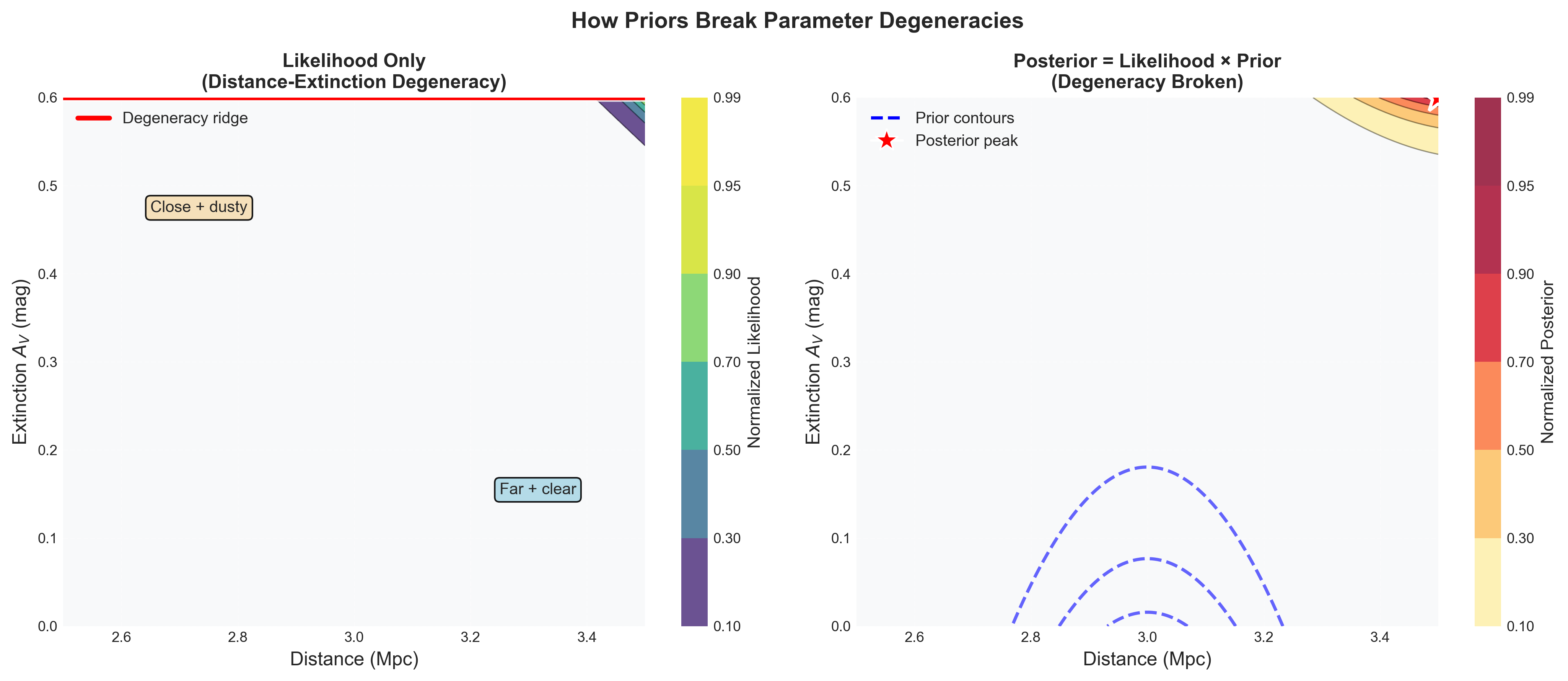
\[ m_{\mathrm{model}}(d, A_V) = M_V(P) + 5 \log_{10}(d / 10~\mathrm{pc}) + A_V. \]

Now the same observed brightness can be explained by a closer, dustier Cepheid or a farther, cleaner one. That is a genuine physical degeneracy, not a numerical inconvenience.

Figure 1: **Distance-extinction degeneracy for a Cepheid-like inference problem.** The elongated ridge shows that many combinations of distance and extinction can reproduce the same brightness. This is the first place students should feel why “just evaluate the posterior on a grid” stops being a satisfying answer: the physics already creates a structured, correlated posterior in only two parameters.

Even this toy extension becomes expensive quickly. A grid with 400 points in $d$ and 400 points in $A_V$ already needs $1.6 \times 10^5$ likelihood evaluations. Add metallicity, intrinsic scatter, a calibration offset, and one nuisance parameter for each observed star, and brute force becomes the bottleneck.

The Curse of Dimensionality

Imagine you want to map out a posterior distribution by evaluating it on a grid. How many grid points do you need?

1D example: To resolve a 1D posterior to reasonable accuracy, you might need $N = 100$ grid points.

2D example: Now you have two parameters. You need $100 \times 100 = 10^4$ evaluations.

3D example: Three parameters $\to$ $100 \times 100 \times 100 = 10^6$ evaluations.

Scaling: For $d$ dimensions, you need $N^d$ evaluations. This is exponential scaling — the curse of dimensionality.

Let’s make this concrete with realistic numbers:

Dimensions	Grid points per dimension	Total evaluations	Time (assuming 1 ms per eval)
1	100	$10^2$	0.1 seconds
2	100	$10^4$	10 seconds
3	100	$10^6$	16 minutes
5	100	$10^{10}$	115 days
10	100	$10^{20}$	3 trillion years
20	100	$10^{40}$	Age of universe $\times 10^{23}$

Even “small” problems with 5-10 parameters become computationally impossible. And many real scientific problems have hundreds or thousands of parameters:

Climate models: ~100 parameters (ocean circulation, cloud physics, aerosols…)
Exoplanet characterization: ~20 parameters per planet (mass, orbit, atmosphere…)
Galaxy formation: ~50 parameters (star formation efficiency, black hole feedback…)
Neural networks: millions to billions of parameters

Grid evaluation simply cannot work.

Connection to Module 1: Volume of High-Dimensional Spheres

Remember the bizarre geometry of high dimensions from Module 1? The volume of a d-dimensional unit sphere is:

\[ V_d = \frac{\pi^{d/2}}{\Gamma(d/2 + 1)} \]

This increases with dimension up to d = 5, then decreases exponentially! By d = 20, essentially all the volume is in the thin shell near the surface.

Most of your grid points are wasted evaluating regions of negligible probability. The probability mass lives in a tiny, weirdly-shaped region of parameter space that you can’t find by uniform sampling.

This is why high-dimensional inference is fundamentally different from low-dimensional intuition.

What About Optimization? Just Find the Peak

maximum a posteriori (MAP) estimation: Finding the parameter values that maximize the posterior distribution. Requires optimization techniques.

uncertainty quantification: The process of determining the degree of uncertainty in parameter estimates, often through credible intervals or posterior distributions.

degeneracies: Situations where different combinations of parameters produce similar model outputs, leading to correlated uncertainties.

evidence: The normalization constant in Bayes’ theorem, representing the total probability of the data under all possible parameter values.

You might think: “Why do I need the full distribution? Just find the maximum of $p(\theta \mid D)$ and report that.”

That reasoning is appealing because optimization is familiar and computationally simpler. But sampling and optimization answer different epistemic questions.

Optimization asks: Which parameter value maximizes the posterior?
Posterior inference asks: Which parameter values remain plausible, and with what relative credibility, given the data and model assumptions?

The second question is scientifically richer because uncertainty, asymmetry, and parameter tradeoffs are often part of the result, not peripheral details.

This is maximum a posteriori (MAP) estimation, and it’s sometimes useful. But you lose crucial information:

1. Uncertainty quantification: The peak tells you nothing about how uncertain you are. Is it a sharp peak (confident) or broad (uncertain)? If you report $\theta = 5.0$ as the MAP estimate, can you distinguish whether your uncertainty is $\pm 0.1$ or $\pm 10$? The peak doesn’t tell you.

2. Asymmetries: The peak might be at $d = 500$ pc, but the distribution could be skewed — maybe $500 \pm 20$ pc toward smaller distances, but $+100$ pc toward larger distances (imagine a long tail from dust extinction uncertainty).

3. Correlations: With multiple parameters, knowing the peak doesn’t tell you about degeneracies. Maybe radius and temperature are correlated — high R and low T give the same luminosity as low R and high T.

4. Model comparison: The evidence $p(D)$ (the denominator in Bayes’ theorem) requires integrating over all parameter values. The peak tells you nothing about this.

5. Propagating uncertainty: If you use your inferred parameters to predict something else, you need the full distribution to get realistic error bars.

The scientific standard: Modern quantitative science does not stop at “best fit” values. It reports credible intervals and posterior structure. Bayesian posteriors do this directly.

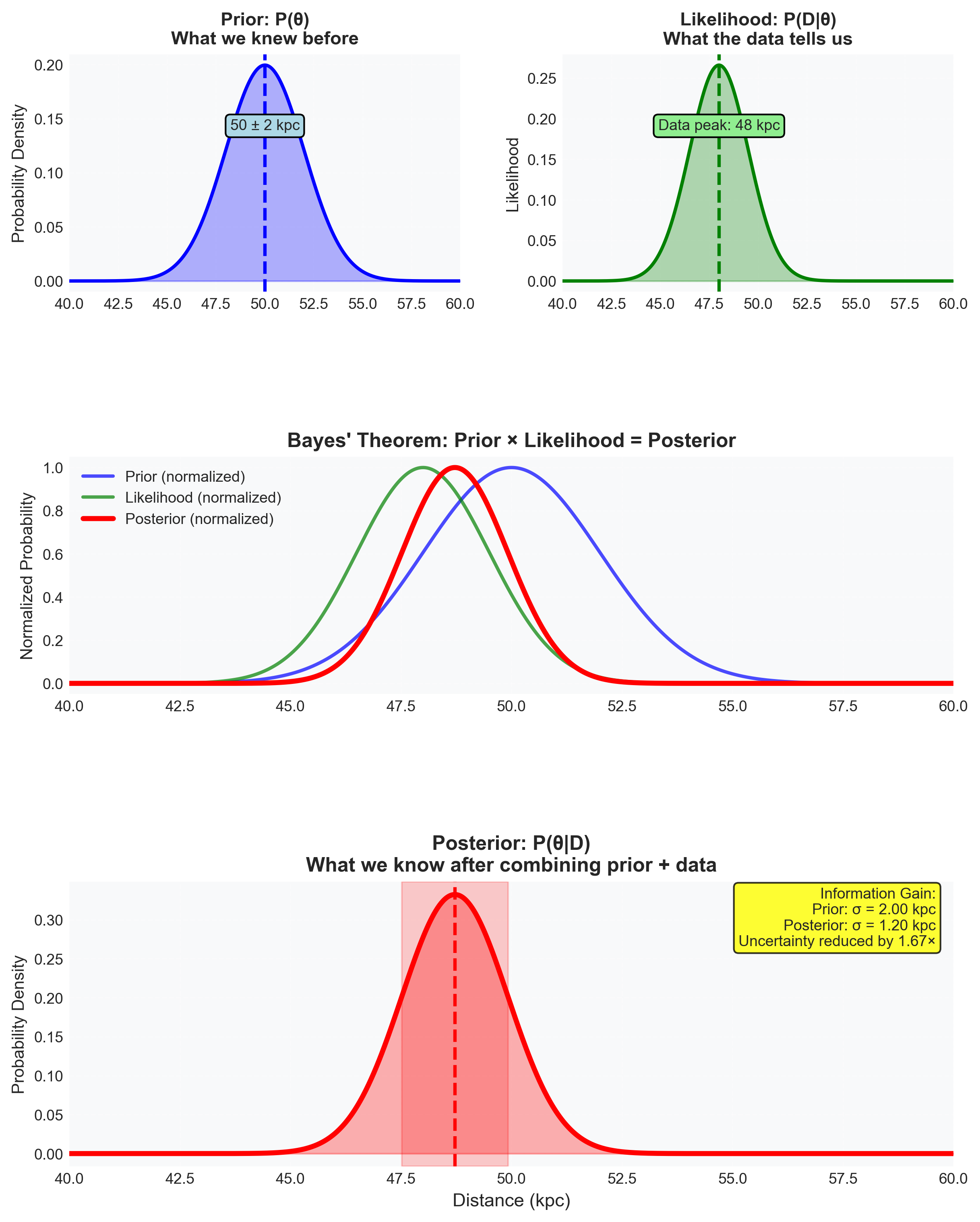
Corrective Example: The Peak Is Not the Posterior

This sentence is wrong:

“The posterior peaks near 323 kpc, so the star is at 323 kpc.”

Why it is wrong:

it ignores the width of the posterior, so it throws away uncertainty
it ignores asymmetry, so it can misreport one-sided uncertainty
it ignores correlations with other parameters in higher dimensions
it treats an inferential distribution as if it were a single fact

The peak is one feature of the posterior. It is not the whole inferential answer.

Figure 2: **A posterior is a full inferential object, not just a location of maximum probability.** Prior, likelihood, and posterior combine into a curve with width and shape. A MAP estimate would choose one location on this curve, but the scientific answer lives in the entire posterior because uncertainty, asymmetry, and later predictions all depend on that full structure.

Epistemic Contrast: Frequentist Testing vs Bayesian Inference

Classical hypothesis testing and Bayesian inference answer different questions.

A p-value asks: If the null hypothesis were true, how surprising would data this extreme be?
A posterior asks: Given the observed data and my modeling assumptions, how plausible are different parameter values or hypotheses?

This lecture focuses on Bayesian inference because it produces the kind of object we want in this course: a probability distribution over unknowns conditioned on data, assumptions, and model structure.

That does not mean frequentist tools are useless. It means they answer a different inferential question than the one we are pursuing here.

What Inference Actually Requires

Now we can state the computational target explicitly.

Everything in the rest of the lecture is in service of the same chain:

\[ \mathbb{E}[f(\theta)\mid D] \;\to\; \int f(\theta)\,p(\theta \mid D)\,d\theta \;\to\; \text{intractable integral} \;\to\; \text{samples} \;\to\; \text{sampler construction}. \]

In science, we rarely want the posterior curve itself. We want derived quantities:

the posterior mean distance,
the probability that a parameter lies in some physically interesting range,
a credible interval,
a prediction under the forward model.

All of these can be written as posterior expectations or posterior integrals. For any function $f(\theta)$,

\[ \mathbb{E}[f(\theta) \mid D] = \int f(\theta)\,\pi(\theta)\,d\theta \]

is the general quantity we want to compute.

For the Cepheid problem, examples include:

$f(d) = d$ for the posterior mean distance,
$f(d) = m_{\mathrm{model}}(d)$ for the mean predicted magnitude,
indicator functions such as $f(d) = \mathbf{1}_{d < 500~\mathrm{kpc}}$ for probabilities of physically relevant events.

This is the conceptual hinge of the lecture:

Inference gives us the posterior $\pi(\theta)$.
Computation must turn that posterior into expectations we can report scientifically.

The Hard Problem

We can often evaluate $\pi(\theta)$ at a chosen point.

What we usually cannot do in moderate or high dimensions is:

integrate $\pi(\theta)$ exactly,
evaluate it accurately on a dense grid,
or draw independent samples from it directly.

That is the tension MCMC resolves.

At this point, all of the standard strategies have failed:

grid evaluation is intractable,
analytic integration is impossible,
and independent sampling is unavailable.

So MCMC is not merely a convenient tool we happen to like. Once direct integration, dense grids, and direct iid (independent and identically distributed) sampling are off the table, constructing a sampler becomes the natural general-purpose strategy if we still want posterior expectations. The natural general-purpose option is to construct a process whose long-run behavior reproduces the posterior. That conceptual move is what defines MCMC.

The Monte Carlo Solution: Sample, Don’t Integrate

Monte Carlo integration: A numerical method that estimates integrals by averaging function values at random samples drawn from a probability distribution.

Sampling distribution: The probability distribution of a statistic (like the mean) computed from random samples of data.

Central Limit Theorem (CLT): A statistical theorem stating that the distribution of the sample mean approaches a normal distribution as the sample size increases, regardless of the original distribution of the data.

Standard error: The standard deviation of a sampling distribution, representing the uncertainty in an estimate due to finite sample size.

Variance reduction techniques: Methods used in Monte Carlo integration to decrease the variance of estimates, improving accuracy without increasing the number of samples.

Here’s where the inference becomes computational. If we had iid samples $\theta_1, \theta_2, \ldots, \theta_N$ drawn from the posterior, then the intractable integral above would become a sample average:

\[ \mathbb{E}[f(\theta) \mid D] = \int f(\theta)\,\pi(\theta)\,d\theta \approx \frac{1}{N}\sum_{i=1}^N f(\theta_i). \]

This is the Monte Carlo idea: replace integration with averaging over samples. It works because an expectation under $\pi(\theta)$ is, by definition, an average of $f(\theta)$ weighted by that distribution; Monte Carlo replaces the exact weighted integral with an empirical average over draws from the same distribution.

If you have $N$ iid samples $\{\theta_1, \theta_2, \ldots, \theta_N\}$ drawn from $p(\theta \mid D)$, then you can estimate many posterior quantities:

Mean: \[\langle \theta \rangle \approx \frac{1}{N} \sum_{i=1}^N \theta_i\]

Variance: \[\text{Var}(\theta) \approx \frac{1}{N} \sum_{i=1}^N (\theta_i - \langle \theta \rangle)^2\]

Credible intervals: Sort the samples and find the 16th and 84th percentiles for a 68% credible interval.

Predictions: For any function $f(\theta)$, estimate its expectation: \[\langle f(\theta) \rangle \approx \frac{1}{N} \sum_{i=1}^N f(\theta_i)\]

The key quantitative fact: For the Monte Carlo estimator

\[ \hat{\mu}_f = \frac{1}{N}\sum_{i=1}^N f(\theta_i) \]

with $\theta_i \stackrel{\text{iid}}{\sim} \pi(\theta)$ and $\sigma_f^2 = \mathrm{Var}[f(\theta)]$, the estimator variance is

\[ \mathrm{Var}(\hat{\mu}_f) = \frac{\sigma_f^2}{N}, \]

so the standard error — the standard deviation of the estimator itself — is

\[ \mathrm{SE}(\hat{\mu}_f) = \frac{\sigma_f}{\sqrt{N}}. \]

The distinction matters:

$\mathrm{Var}(\hat{\mu}_f)$ tells you how the estimator’s variance shrinks with sample size,
$\mathrm{SE}(\hat{\mu}_f)$ is the uncertainty scale for the estimator itself.

The Central Limit Theorem implies that the sampling distribution of the estimator has variance $\sigma_f^2/N$, so its standard deviation (the standard error) scales as $\sigma_f/\sqrt{N}$.

Important: Monte Carlo Scaling with Dimension

In the iid Monte Carlo setting, the standard-error rate is $O(N^{-1/2})$, and that rate does not itself deteriorate exponentially with dimension. However, dimension can still matter through the constant $\sigma_f$, through geometric concentration, and through how difficult it is to obtain representative samples for the integrand you care about.

To gain one more decimal place of accuracy, you need about $100 \times$ more samples. That is slow convergence. But it is still fundamentally better than dense-grid integration in high dimensions, where the cost typically grows exponentially with the number of parameters.

This is revolutionary. Grid evaluation scales exponentially with dimension $(N^d)$. By contrast, iid Monte Carlo has an $O(N^{-1/2})$ convergence rate that does not itself worsen exponentially with dimension.

Connection to Module 1: Law of Large Numbers and CLT

Everything we’re doing rests on two facts from Module 1:

If ${\theta_i}$ are independent samples from a distribution with finite variance, then the Law of Large Numbers says

\[ \frac{1}{N} \sum_{i=1}^N f(\theta_i) \to \mathbb{E}[f(\theta)] \quad \text{as } N \to \infty, \]

which explains why sample averages estimate expectations.

The Central Limit Theorem then quantifies the remaining uncertainty: for large $N$, the estimator $\hat{\mu}_f$ fluctuates around the true expectation with standard error approximately

\[ \frac{\sigma_f}{\sqrt{N}}. \]

That is why Monte Carlo works: expectations become sample averages, and the uncertainty of those averages shrinks like $1/\sqrt{N}$. In MCMC the samples are correlated, so the same logic applies but with an effective sample size smaller than $N$, which we will quantify later.

But here’s the catch: We do not have a machine that hands us independent samples from $\pi(\theta) = p(\theta \mid D)$. We can evaluate the posterior at points we choose, but evaluation is not the same as sampling.

So the problem changes form:

How do we generate samples from a distribution we can evaluate but cannot sample from directly?

This is where Markov Chain Monte Carlo enters. It’s a method to generate samples from a very broad class of target distributions by constructing a Markov chain that explores parameter space.

What We Just Learned

At the Observable $\to$ Model $\to$ Inference $\to$ Computation level, Part 1 identifies the bottleneck. The posterior is the right inferential object, but direct evaluation fails in realistic dimensions. MCMC is the computational response to that failure.

Part 2: Markov Chains — The Mathematical Foundation

The Core Idea: Build a Stochastic Process

Because direct independent sampling from $\pi(\theta) = p(\theta \mid D)$ is unavailable, we replace it with a stochastic process that produces dependent samples whose long-run frequencies still match the posterior.

This is the key conceptual relaxation. If independent samples are impossible, then we must allow dependence between successive samples. The simplest structure that introduces dependence without becoming hopelessly complicated is a Markov process: the next state depends only on the current one.

That is why Markov chains appear here. They are not arbitrary decoration. They are the minimal relaxation of independence that still gives us a tractable way to construct a sampler.

Instead of trying to sample directly from $p(\theta \mid D)$, we’ll build a stochastic process (a Markov chain) that:

Starts from any initial $\theta_0$
Takes random steps through parameter space
Gradually “forgets” where it started
Eventually produces samples distributed according to $p(\theta \mid D)$

Think of it like a random walker wandering around parameter space. We’ll design the rules of walking so that after sufficient wandering, the walker spends time in each region proportional to $p(\theta \mid D)$.

If $p(\theta \mid D)$ is high in some region, the walker visits often. If $p(\theta \mid D)$ is low, the walker rarely goes there. The stationary distribution of the random walk is the posterior.

Markov Chains: Formal Definition

stochastic process: A collection of random variables indexed by time or space, representing a system that evolves randomly over time. Markov property: The property of a stochastic process where the future state depends only on the present state, not on the sequence of events that preceded it. transition kernel: A function that defines the probabilities of moving from one state to another in a Markov chain. stationary distribution: A probability distribution that remains unchanged as the system evolves over time in a Markov chain. ergodicity: A property of a Markov chain where it is possible to reach any state from any other state, ensuring that long-term averages converge to expected values.

A Markov chain is not yet an inference method. It is a type of stochastic process. We choose it because it is the simplest sequential mechanism rich enough to produce dependent samples with a controllable long-run distribution.

Its defining property is simple:

the next state depends only on the current state, not on the full past history.

In symbols,

\[ p(\theta_{t+1} | \theta_t, \theta_{t-1}, \theta_{t-2}, ..., \theta_0) = p(\theta_{t+1} | \theta_t) \]

This is the Markov property: the future depends on the present, not the past. Once that idea is clear, we can introduce the next crucial object: the transition kernel $T(\theta' \mid \theta)$, which tells us how the chain moves through parameter space.

Physical Intuition: Random Walk

Imagine a drunk walker on a street. At each time step, they randomly choose to take a step left or right. Where they go next depends only on where they are now, not how they got there. That’s the Markov property.

In parameter space, $\theta$ is the walker’s current location. The transition kernel tells you the probability of moving to each possible new location $\theta'$.

Transition Kernels

The dynamics of a Markov chain are defined by the transition kernel (or transition probability):

\[ T(\theta' | \theta) \]

This is the probability density of moving to $\theta'$ given that you’re currently at $\theta$. It must satisfy:

\[ \int T(\theta' | \theta) \, d\theta' = 1 \]

for all $\theta$ (probabilities must sum to 1).

Given a starting distribution $p_0(\theta)$, the distribution after one step is:

\[ p_1(\theta') = \int p_0(\theta) T(\theta' | \theta) \, d\theta \]

After $t$ steps:

\[ p_t(\theta') = \int p_{t-1}(\theta) T(\theta' | \theta) \, d\theta \]

Question: Can we design $T$ such that $p_t(\theta)$ converges to our target distribution $\pi(\theta) = p(\theta \mid D)$ as $t \to \infty$?

Answer: Yes! But we need two conditions:

Stationarity: The target distribution $\pi$ must be stationary with respect to $T$.
Ergodicity: The chain must be able to explore the entire parameter space.

Stationarity: The Distribution Must Be Preserved

A distribution $\pi(\theta)$ is stationary with respect to $T$ if applying the transition kernel doesn’t change it:

\[ \int \pi(\theta) T(\theta' | \theta) \, d\theta = \pi(\theta') \]

What it is: If the Markov chain is distributed according to $\pi$, then after one more step, it’s still distributed according to $\pi$. The distribution is an equilibrium of the dynamics.

Physical analogy: A gas in thermal equilibrium. Molecules are constantly moving and colliding, but the overall distribution (Boltzmann distribution) doesn’t change. Individual states change, but the probability distribution is stationary.

These two ideas play different roles:

Stationarity tells us the target distribution is preserved by the dynamics.
Ergodicity tells us the chain can actually find and explore that distribution from arbitrary starting points.

A chain can have the correct stationary distribution on paper and still be scientifically useless if it cannot explore the relevant regions of parameter space.

Ergodicity: The Chain Must Explore Everywhere

Stationarity means $\pi$ is preserved if you start from it. But how do we get there from an arbitrary starting point $\theta_0$?

We need ergodicity: The chain must be able to reach any state from any other state in finite time. Formally, ergodicity requires:

1. Irreducibility: Every state is accessible from every other state (there are no isolated regions).

2. Aperiodicity: The chain doesn’t get stuck in cycles. (E.g., don’t alternate deterministically: left, right, left, right forever.)

Connection to Module 3: Phase Space and Ergodicity

In Module 3 (statistical mechanics), you learned the ergodic hypothesis: Time averages equal ensemble averages. A system exploring its phase space eventually visits all accessible microstates with frequency proportional to their statistical weight.

The same principle applies here. Your Markov chain explores parameter space, eventually visiting each region with frequency proportional to $\pi(\theta) = p(\theta \mid D)$.

Module 3: Ergodicity lets us replace ensemble averages (over all possible configurations) with time averages (following one trajectory).
Module 5: Ergodicity lets us replace ensemble sampling (drawing independent samples from $\pi$) with sequential sampling (following one Markov chain).

It’s the same concept applied to probability distributions instead of physical systems.

The Ergodic Theorem: If a Markov chain is ergodic and has stationary distribution $\pi$, then for any function $f(\theta)$:

\[ \lim_{N \to \infty} \frac{1}{N} \sum_{t=1}^N f(\theta_t) = \int f(\theta) \pi(\theta) \, d\theta \]

Time averages along the chain converge to expectations under $\pi$. This is how MCMC works: run the chain for a long time, then use the samples to estimate expectations.

Detailed Balance: A Sufficient Condition for Stationarity

At this point we need a design test. A chain that merely “moves around” parameter space is not enough. A random walk could easily settle into the wrong distribution. We need a condition we can verify mathematically that guarantees the chain targets the right long-run distribution.

Here is the failure mode to keep in mind. Suppose we design a random walk that proposes steps and always accepts them. It will certainly explore parameter space, but it will not generally spend time in each region proportional to $\pi(\theta)$. In fact, for a symmetric proposal on a bounded space, it tends to behave much more like uniform exploration than posterior sampling.

So “motion” is not enough. We need a correction mechanism that reshapes the dynamics so the chain has the right equilibrium distribution. Detailed balance is the first clean way to express that requirement mathematically.

Detailed balance is not the only possible route to stationarity, but it is a powerful sufficient condition because it is local, checkable, and easy to build into an algorithm.

We need to design a transition kernel $T$ that has $\pi$ as its stationary distribution. There’s a powerful sufficient condition called detailed balance (also called microscopic reversibility):

\[ \pi(\theta) T(\theta' | \theta) = \pi(\theta') T(\theta | \theta') \]

In words: the probability flow from $\theta$ to $\theta'$ equals the flow from $\theta'$ back to $\theta$ when both are drawn from $\pi$.

Why does detailed balance imply stationarity? Here’s the key insight:

Detailed balance is a sufficient condition for stationarity. To see why, assume detailed balance holds and integrate both sides over $\theta$:

\[ \int \pi(\theta) T(\theta' | \theta) \, d\theta = \int \pi(\theta') T(\theta | \theta') \, d\theta \]

The right side factors since $\pi(\theta')$ doesn’t depend on the integration variable:

\[ \text{RHS} = \pi(\theta') \int T(\theta | \theta') \, d\theta = \pi(\theta') \times 1 = \pi(\theta') \]

(The integral equals 1 because T is a probability density in its first argument.)

The left side is exactly the definition of how the distribution evolves forward one step:

\[ \text{LHS} = \int \pi(\theta) T(\theta' | \theta) \, d\theta \]

This integral gives you the probability at $\theta'$ after one transition starting from $\pi$. Since $\text{LHS} = \text{RHS} = \pi(\theta')$, we’ve shown that starting from distribution $\pi$ produces distribution $\pi$ after one step. The distribution is stationary.

Physical Intuition: Equilibrium Flow

Imagine a fluid flowing between two containers. Detailed balance says: At equilibrium, the flow rate from container A to B equals the flow rate from B to A.

If inflow equals outflow for every pair of states, then the overall distribution doesn’t change. That’s stationarity.

In statistical mechanics, this is called microscopic reversibility: At thermal equilibrium, every microscopic process and its reverse occur at equal rates. This is a fundamental principle of thermodynamics that MCMC inherits.

Connection to Module 3: Statistical Mechanics

The detailed balance equation is identical to the condition for thermal equilibrium in statistical mechanics:

\[ \rho_i W_{i \to j} = \rho_j W_{j \to i} \]

where $\rho_i$ is the probability of microstate $i$ and $W_{i \to j}$ is the transition rate from $i$ to $j$.

For a Hamiltonian system in thermal equilibrium at temperature T, the Boltzmann distribution:

\[ \rho_i \propto e^{-E_i / k_B T} \]

satisfies detailed balance with respect to the dynamics of the system. This is why thermalization works — microscopic reversibility guarantees that systems evolve toward the Boltzmann distribution.

MCMC uses the same mathematical structure to guarantee that your sampler evolves toward the posterior distribution $p(\theta \mid D)$. It’s not mere analogy — they’re the same theorem applied to different systems.

Now we have our blueprint:

Choose a target distribution $\pi(\theta) = p(\theta \mid D)$.
Design a transition kernel $T$ that satisfies detailed balance with respect to $\pi$.
The Markov chain will converge to $\pi$ (if ergodic).
Run the chain, collect samples, estimate expectations

The question: How do we actually construct such a $T$? That’s where Metropolis-Hastings comes in.

What We Just Learned

Markov chains supply the mechanism. If we can build dynamics whose stationary distribution is the posterior, then time averages along the chain become posterior expectations. Detailed balance tells us how to make that construction mathematically legitimate.

Part 3: The Metropolis-Hastings Algorithm

Where We Are

The journey so far: In Part 1, we discovered that grid evaluation fails exponentially with dimension — the curse of dimensionality. In Part 2, we learned that Markov chains offer a solution: build a random walk that explores parameter space and, under the right conditions, produces samples from a broad class of target distributions, justified by ergodicity and detailed balance.

Now in Part 3: We’ll construct the specific algorithm that makes this work — the Metropolis-Hastings sampler, a general-purpose method for sampling from complicated target distributions when direct iid sampling is unavailable.

The Construction: Proposal + Accept/Reject

Here’s the brilliant idea due to Metropolis et al. (1953) and generalized by Hastings (1970):

The More You Know: The Manhattan Project Origins of MCMC

The Metropolis algorithm has remarkable origins. In the early 1950s, Nicholas Metropolis, Arianna Rosenbluth, Marshall Rosenbluth, Augusta Teller, and Edward Teller were working at Los Alamos National Laboratory on the hydrogen bomb project. They needed to understand how atoms in materials would behave under extreme conditions — millions of degrees, enormous pressures — but they couldn’t build physical experiments to measure this (too dangerous and expensive). They also couldn’t solve the equations analytically (too many particles, too complex).

Their insight: Simulate the particles computationally. But even simulation was a challenge — how do you sample from the Boltzmann distribution at high temperature without computing the partition function (which requires summing over all possible states)? Rosenbluth had the key idea: Use a Markov chain with accept/reject steps based on energy differences. The normalization constant cancels out!

The first calculation ran on MANIAC I (Mathematical Analyzer Numerical Integrator and Computer), one of the earliest digital computers. The problem: 224 particles interacting via Lennard-Jones potential. The computation took hours. Today your laptop could do it in seconds.

The profound irony: A method developed to understand nuclear weapons physics has become one of the most important tools in peaceful science — from astronomy to medicine to machine learning. Computational methods developed for destruction now help us understand the universe.

The original 1953 paper is a model of clarity and is still worth reading. Metropolis’s name appears first, but by alphabetical convention — the method was really a collaborative effort. Augusta Teller (Edward Teller’s wife) and Arianna Rosenbluth are sometimes forgotten in historical accounts, yet another example of how women’s contributions to computational science have been underrecognized.

Separate the transition kernel into two parts:

Proposal distribution $Q(\theta' \mid \theta)$: generates a candidate new state $\theta'$ given current state $\theta$
Acceptance probability $\alpha(\theta' \mid \theta)$: probability of accepting the proposal

For $\theta' \neq \theta$, the accepted-move component of the transition kernel is:

\[ T(\theta' \mid \theta) = Q(\theta' \mid \theta)\,\alpha(\theta' \mid \theta) \]

The full kernel also includes a self-transition at $\theta' = \theta$ that collects the rejected proposals. In other words, “reject and stay where you are” is part of the Markov dynamics itself, not an implementation afterthought.

Operational View: What MCMC Actually Does

MCMC constructs a sequence

\[ \theta_0 \to \theta_1 \to \theta_2 \to \cdots \]

that wanders through parameter space. The samples are not independent. Instead, after burn-in, the fraction of time the chain spends in any region $R$ approximates

\[ \int_R \pi(\theta)\,d\theta. \]

That is why posterior expectations become sample averages. We are not simulating a search for the best point. We are simulating a dynamical system whose long-run visitation frequencies encode the posterior.

The algorithm:

Start at some $\theta_0$ (anywhere in parameter space)
For $t = 0, 1, 2, ..., N-1$:
- Propose: Draw $\theta'$ from $Q(\theta' \mid \theta_t)$
- Evaluate: Compute acceptance probability $\alpha(\theta' \mid \theta_t)$
- Decide:
  - With probability $\alpha$, accept: $\theta_{t+1} = \theta'$
  - With probability $1-\alpha$, reject: $\theta_{t+1} = \theta_t$ (stay put)
Return samples $\{\theta_1, \theta_2, \ldots, \theta_N\}$

The magic is in step 2: How do we choose $\alpha$ to satisfy detailed balance?

Pause and Predict

Before we derive the acceptance probability, take a moment to think:

Given that we want detailed balance $\pi(\theta) T(\theta' \mid \theta) = \pi(\theta') T(\theta \mid \theta')$, and we’ve decided $T = Q \times \alpha$, what constraints must $\alpha$ satisfy?

Write down your answer before reading on:

Should $\alpha$ depend on both $\theta$ and $\theta'$, or just one?
If $\theta'$ has higher posterior probability than $\theta$, should we always accept?
If $\theta'$ has lower posterior probability, should we always reject?
What role does the proposal distribution $Q$ play?

Think about it for 30 seconds, then continue. The derivation will be more meaningful if you’ve wrestled with the problem first.

Deriving the Acceptance Probability

We want:

\[ \pi(\theta) T(\theta' | \theta) = \pi(\theta') T(\theta | \theta') \]

Substituting $T = Q\alpha$ where $Q$ is the proposal and $\alpha$ is the acceptance probability:

\[ \pi(\theta) Q(\theta' | \theta) \alpha(\theta' | \theta) = \pi(\theta') Q(\theta | \theta') \alpha(\theta | \theta') \]

Rearrange:

\[ \frac{\alpha(\theta' | \theta)}{\alpha(\theta | \theta')} = \frac{\pi(\theta') Q(\theta | \theta')}{\pi(\theta) Q(\theta' | \theta)} \]

Define the acceptance ratio:

\[ r = \frac{\pi(\theta') Q(\theta | \theta')}{\pi(\theta) Q(\theta' | \theta)} \]

When $\pi$ is the posterior: write \[\pi(\theta) \propto p(D\mid\theta)p(\theta).\]

Then

\[ r \;=\; \frac{\pi(\theta')\,Q(\theta\mid\theta')}{\pi(\theta)\,Q(\theta'\mid\theta)} \;=\; \frac{p(D\mid\theta')\,p(\theta')}{p(D\mid\theta)\,p(\theta)} \cdot \frac{Q(\theta\mid\theta')}{Q(\theta'\mid\theta)}, \]

so the evidence $p(D)$ cancels because it is constant in $\theta$.

We need $\alpha(\theta' \mid \theta)$ and $\alpha(\theta \mid \theta')$ to have ratio $r$. A simple choice that works:

\[ \alpha(\theta' | \theta) = \min(1, r) = \min\left(1, \frac{\pi(\theta') Q(\theta | \theta')}{\pi(\theta) Q(\theta' | \theta)}\right) \]

Verification: Let

\[ R = \frac{\pi(\theta')Q(\theta \mid \theta')}{\pi(\theta)Q(\theta' \mid \theta)} \]

If $R \geq 1$: $\alpha(\theta' \mid \theta) = 1$, $\alpha(\theta \mid \theta') = 1/R \leq 1$. Ratio: $1/(1/R) = R$.
If $R < 1$: $\alpha(\theta' \mid \theta) = R$, $\alpha(\theta \mid \theta') = 1$. Ratio: $R/1 = R$.

Either way, the ratio condition is satisfied, so detailed balance holds!

Interpretation:

If $\theta'$ has higher posterior probability than $\theta$ $(R > 1)$, always accept.
If $\theta'$ has lower posterior probability $(R < 1)$, accept with probability $R$.

The accept/reject rule does something subtle and important:

it favors moves toward higher posterior density,
but it does not force greedy ascent.

That is exactly why MCMC samples a distribution instead of performing optimization. Occasional moves into lower-probability regions are not mistakes; they are part of correctly representing posterior uncertainty.

What Problem Is Metropolis-Hastings Solving?

The goal is not to find the best point. The goal is to construct a stochastic process whose long-run behavior reproduces the posterior distribution.

The proposal creates motion.
The accept/reject step corrects that motion so the chain does not wander arbitrarily.
Detailed balance is the mathematical guarantee that the long-run sample frequencies match the target posterior.

The More You Know: Why “$\min(1, r)$” Works

You might wonder: Why specifically $\min(1, r)$? Could we use other acceptance probabilities?

Yes. Any choice of $\alpha$ that satisfies the ratio condition works. But $\min(1, r)$ is optimal in a precise sense: it maximizes the acceptance rate while satisfying detailed balance.

Proof sketch: If we used $\alpha(\theta' \mid \theta) = r/(1+r)$, we’d accept less often but still satisfy detailed balance. However, lower acceptance means slower exploration and higher autocorrelation. The Metropolis-Hastings choice $\min(1, r)$ accepts as often as possible while maintaining detailed balance.

This is an example of the “Barker acceptance” vs. “Metropolis acceptance” distinction. Metropolis is provably more efficient.

Proposal Distributions: Symmetric vs. Asymmetric

The acceptance probability depends on the proposal distribution $Q$. Two important cases:

Symmetric proposals: $Q(\theta' \mid \theta) = Q(\theta \mid \theta')$.

Example — Gaussian random walk (symmetric in $\theta$): \[ \theta' \sim \mathcal{N}(\theta;\,\Sigma)\quad\Longleftrightarrow\quad \theta'=\theta+\varepsilon,\;\varepsilon\sim\mathcal{N}(0,\Sigma). \]

For symmetric $Q$, the $Q$-terms cancel and \[ \alpha=\min\!\left(1,\frac{\pi(\theta')}{\pi(\theta)}\right). \]

Here you can evaluate $\pi$ using only log-likelihood + log-prior; any constant normalizer cancels. This is the Metropolis algorithm (the original 1953 version). You only need to evaluate the ratio of posterior probabilities.

Asymmetric proposals: $Q(\theta' \mid \theta) \neq Q(\theta \mid \theta')$

Example: Propose $\theta'$ by drawing from the prior $p(\theta)$.

Then: \[\alpha = \min\left(1, \frac{\pi(\theta') Q(\theta | \theta')}{\pi(\theta) Q(\theta' | \theta)}\right)\]

You need the full ratio including the $Q$ terms. This is the Metropolis-Hastings algorithm (Hastings 1970 generalization).

Practical Tip: Start Simple

For most problems, start with a symmetric Gaussian random walk proposal: \[\theta' = \theta_t + \epsilon, \quad \epsilon \sim \mathcal{N}(0, \sigma^2 I)\]

This is simple to implement and works well if you tune $\sigma$ appropriately. Once you have that working, you can try fancier proposals if needed.

Tuning the Proposal: The Art of Step Size

The proposal distribution Q determines how the chain explores. A crucial parameter is the step size (scale of proposals).

Too small: Proposals are always accepted $(\alpha \approx 1)$, but you take tiny steps. The chain explores very slowly. High autocorrelation between successive samples.

Too large: Proposals often land in low-probability regions. High rejection rate $(\alpha \approx 0)$. The chain stays stuck in one place most of the time. Again, slow exploration.

Just right: Moderate acceptance rate (typically 20-50%). The chain explores efficiently, taking substantial steps while still accepting frequently enough.

Optimal Acceptance Rates

For high-dimensional problems with Gaussian targets and Gaussian proposals, there’s a beautiful theory (Roberts & Rosenthal 2001):

Optimal acceptance rate: $\sim 23.4\%$ as dimension $d \to \infty$

This balances:

Acceptance rate (how often you move)
Step size (how far you move when accepted)

In practice, aim for:

1D problems: 40-50% acceptance
Moderate dimensions (2-20): 25-40% acceptance
High dimensions (>20): 20-30% acceptance

If your acceptance rate is outside these ranges, adjust your proposal scale $\sigma$:

Too high acceptance (>60%)? Increase $\sigma$
Too low acceptance (<15%)? Decrease $\sigma$

Adaptive tuning: In practice, you might run the chain for a burn-in period, monitor the acceptance rate, and adjust $\sigma$. Common strategy:

Run 1000 steps (burn-in)
If acceptance rate > 50%, multiply $\sigma$ by 1.2
If acceptance rate < 20%, divide $\sigma$ by 1.2
Repeat until acceptance rate is in target range

Once tuned, fix the proposal and run your production chain. (Don’t keep adapting during production — this violates the Markov property and detailed balance.)

From Likelihood to Log-Posterior Code

This is the bridge students usually need made explicit. For any Bayesian model, the implementation pipeline is:

Write the forward model that predicts observables from parameters.
Write the log-likelihood from your noise model.
Write the log-prior from your scientific assumptions and parameter bounds.
Add them to get the unnormalized log-posterior:

\[ \log \pi(\theta) = \log p(D \mid \theta) + \log p(\theta) + C, \]

where the constant $C = -\log p(D)$ can be ignored.

In practice, this is the computational object nearly everything reduces to:

def log_posterior(theta):
    return log_likelihood(theta) + log_prior(theta)

MCMC algorithms work by comparing this quantity between the current and proposed states. Ratios in probability space become subtraction in log space, which is why log-space arithmetic is not optional numerical polish but part of the method itself.

Run the sampler on differences in $\log \pi(\theta)$ between the current and proposed states.

That is the whole computational bridge:

\[ \text{physics} \to \text{likelihood} \to \log \text{posterior} \to \text{proposal loop} \to \text{samples}. \]

Purpose: the code below is a minimal reusable Metropolis-Hastings skeleton.

Inputs: a function that evaluates the unnormalized log-posterior, a proposal rule, an initial parameter vector, and the number of samples.

Outputs: a Markov chain of sampled parameter states plus the acceptance rate.

Common pitfall: on rejection, you must still record the current state again. Rejected proposals do not disappear from the chain; “staying put” is part of the Markov process.

Minimal Sampler Skeleton

import numpy as np  # for np.log, np.random.uniform, array handling

def metropolis_hastings(log_posterior, proposal, theta_init, n_samples):
    """
    Generic Metropolis-Hastings MCMC sampler.
    
    Parameters:
    -----------
    log_posterior : function
        Computes log pi(theta) (log posterior probability). Return the unnormalized log posterior: log p(D|theta) + log p(theta). Do not include log p(D); it is a constant and cancels in MH.
    proposal : function  
        Generates theta_prime given theta. Returns theta_prime and log_Q_ratio = log Q(theta|theta_prime) - log Q(theta_prime|theta) (order matters)
    theta_init : array
        Initial parameter values
    n_samples : int
        Number of MCMC samples to generate
    
    Returns:
    --------
    chain : array (n_samples, n_params)
        MCMC samples
    acceptance_rate : float
        Fraction of accepted proposals
    """
    
    theta = theta_init.copy()
    chain = np.zeros((n_samples, len(theta)))
    n_accepted = 0
    
    log_pi_current = log_posterior(theta)
    
    for i in range(n_samples):
        # 1. Propose new state
        theta_proposed, log_Q_ratio = proposal(theta)
        
        # 2. Evaluate posterior at proposed state
        log_pi_proposed = log_posterior(theta_proposed)
        
        # 3. Compute acceptance probability (in log space!)
        log_alpha = log_pi_proposed - log_pi_current + log_Q_ratio
        
        # 4. Accept or reject
        if np.log(np.random.uniform()) < log_alpha:
            # Accept
            theta = theta_proposed
            log_pi_current = log_pi_proposed
            n_accepted += 1
        # If rejected, theta stays the same (automatic in this code structure)
        
        # 5. Store sample
        chain[i] = theta
    
    acceptance_rate = n_accepted / n_samples
    return chain, acceptance_rate

Key implementation details:

Work in log space

Purpose: show why a sampler evaluates log-probabilities instead of raw probabilities. Inputs: two extremely small probability values. Output: a finite log-ratio that can still be compared numerically. Pitfall: direct probabilities underflow to zero, so ratio calculations become undefined.

# Direct space: numerical disaster
p1 = 1e-1000  # Underflows to 0!
p2 = 1e-1001  # Also underflows to 0!
ratio = p2 / p1  # 0/0 = NaN. Game over.

# Log space: works perfectly  
log_p1 = -1000 * np.log(10)  # ~-2302.6
log_p2 = -1001 * np.log(10)  # ~-2305.0  
log_ratio = log_p2 - log_p1  # -2.3 (a perfectly fine number!)
# If log_p = -1000, then p = exp(-1000) = 0 (underflow!)
# But log_p = -1000 is a perfectly fine number to work with.

Proposal functions

Purpose: generate a candidate move for a symmetric random-walk sampler. Input: current parameter vector and a proposal scale. Output: proposed parameter vector plus the proposal-density correction term. Pitfall: if the proposal is not actually symmetric, you cannot set log_Q_ratio = 0.0.

def gaussian_proposal(theta, sigma=1.0):
    theta_new = theta + np.random.normal(0, sigma, size=len(theta))
    log_Q_ratio = 0.0  # Symmetric, so Q(theta|theta_prime)/Q(theta_prime|theta) = 1
    return theta_new, log_Q_ratio

Acceptance decision: Compare log(uniform random) to $\log \alpha$ instead of comparing a uniform random draw to $\alpha$. This avoids exponentiating large negative numbers. (Use unnormalized log posterior: loglike + logprior; do not add log p(D).)

What About the Normalization Constant?

Recall: we only need $\pi(\theta)$ up to proportionality; this section shows explicitly how $p(D)$ cancels from the MH acceptance ratio.

Remember Bayes’ theorem:

\[ p(\theta | D) = \frac{p(D | \theta) p(\theta)}{p(D)} \]

The denominator $p(D)$ is often intractable (that’s why we’re doing MCMC in the first place!). But look at the acceptance probability:

\[ \alpha = \min\left(1, \frac{p(\theta' | D)}{p(\theta | D)}\right) = \min\left(1, \frac{p(D | \theta') p(\theta') / p(D)}{p(D | \theta) p(\theta) / p(D)}\right) \]

The $p(D)$ terms cancel! You only need:

\[ \alpha = \min\left(1, \frac{p(D | \theta') p(\theta')}{p(D | \theta) p(\theta)}\right) \]

Profound implication: MCMC only requires evaluating the unnormalized posterior (likelihood $\times$ prior). You never need the evidence $p(D)$.

This is why MCMC works for arbitrarily complex models. As long as you can evaluate $p(D \mid \theta)$ (your likelihood/model) and $p(\theta)$ (your prior), you can sample from the posterior.

What We Just Learned

Metropolis-Hastings turns posterior evaluation into posterior sampling. You do not need the normalization constant, only relative posterior weight. That is the key computational breakthrough.

Part 4: Practical Diagnostics — Has Your Chain Converged?

Where We Are

The journey so far: Part 1 showed us the crisis (grid evaluation fails). Part 2 gave us the theory (Markov chains, detailed balance, ergodicity). Part 3 delivered the algorithm (Metropolis-Hastings acceptance criterion).

Now in Part 4: We face the practitioner’s challenge — you’ve run your MCMC code and it produced numbers, but are they trustworthy? How do you know the chain has converged? This part gives you the diagnostic tools to answer that critical question.

You’ve run your MCMC algorithm for N steps. You have N samples. Now the crucial question: Are these samples from the posterior?

The ergodic theorem says the chain eventually converges to $\pi$. But how long is “eventually”? If you haven’t run long enough, your samples don’t represent the posterior — they’re still biased toward your starting point.

This is the burn-in problem: Early samples are not from $\pi$. You need to discard them.

Convergence is therefore not something you “prove” from a single plot. It is a judgment built from several pieces of evidence that all point in the same direction: stationarity, mixing, agreement across chains, and enough effectively independent samples.

Visual Diagnostic: Trace Plots

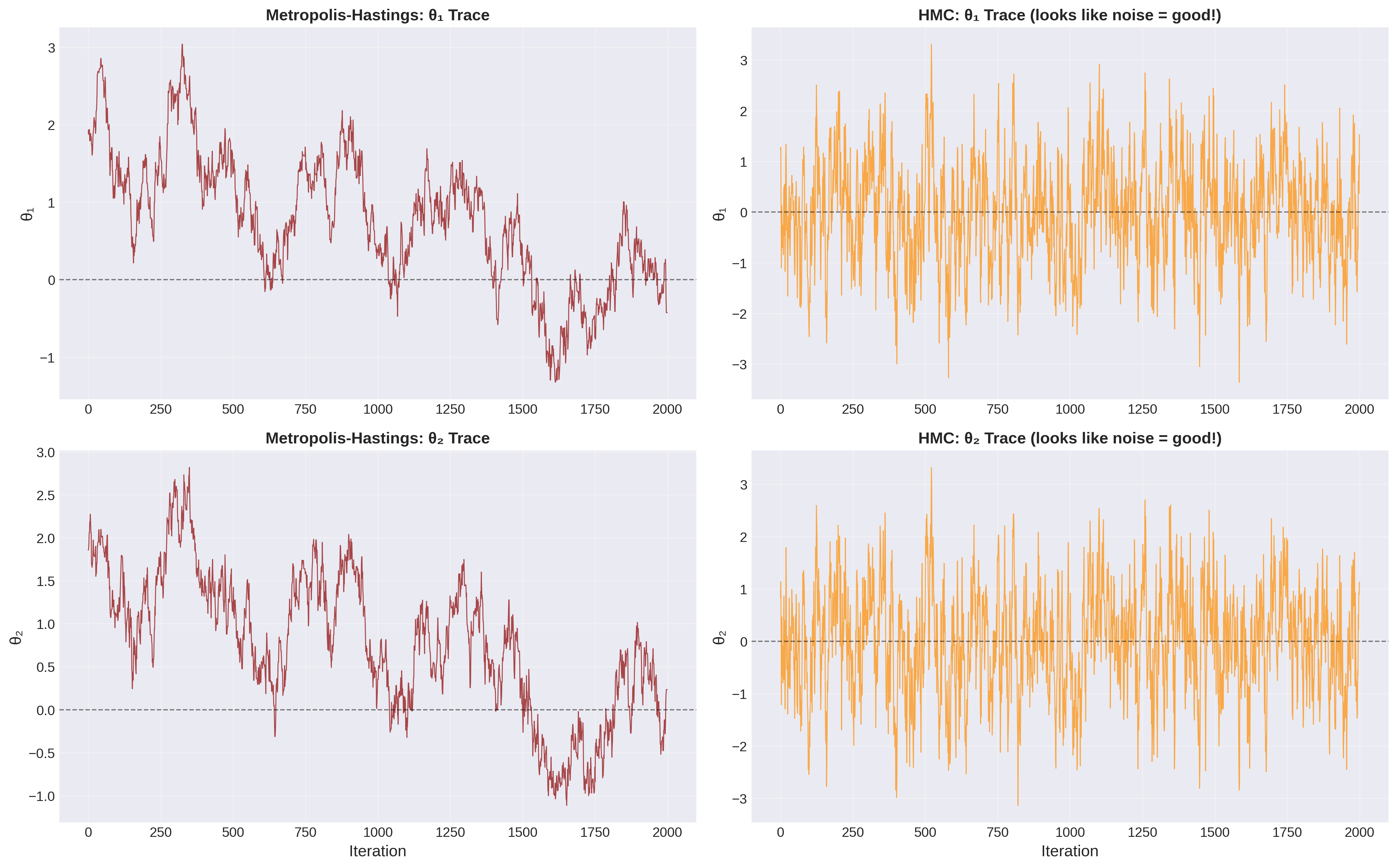
The first and most important diagnostic: Plot your samples over time.

Figure 3: **Representative trace-plot behaviors for MCMC.** A good trace plot looks like stationary, overlapping noise after burn-in, while problematic chains show drift or long sticky plateaus. This is the visual version of the convergence question students should ask before trusting any posterior summary.

A trace plot shows $\theta_t$ vs. $t$. What to look for:

Good signs:

Looks like random noise around a stable mean
No trends (increasing or decreasing)
No periodic oscillations
Mixes well (explores the full range rapidly)
Multiple chains from different starting points overlap

Bad signs:

Systematic trend (chain hasn’t equilibrated)
Stuck in one region for a long time (mixing poorly)
Periodic oscillations (not ergodic, perhaps?)
Multiple chains give different distributions (not converged)

Example: What Trace Plots Tell You

Imagine three scenarios:

Scenario 1: Not burned in

Iteration:  0 -------- 5000 -------- 10000
Parameter:  10         ↓               5
            |          ↓               ↓
            |          ↓               ⟷
            |          ↓               ⟷

Clear downward trend. The chain started at $\theta = 10$ and is still drifting toward the high-probability region near $\theta = 5$. Solution: discard the first $\sim 7000$ samples.

Scenario 2: Well-mixed, converged

Iteration:  0 -------- 5000 -------- 10000
Parameter:  ⟷          ⟷               ⟷
            ⟷          ⟷               ⟷
            5          5               5

Rapid fluctuations around stable mean. Looks like white noise. This is what you want!

Scenario: 3 Stuck (poor mixing)

Iteration:  0 -------- 5000 -------- 10000  
Parameter:  5555555555 4444444444     6666666

Chain stays at one value for thousands of iterations, then jumps. The proposals are being rejected too often (step size too large?) or the posterior is multimodal (chain is trapped in one mode). Bad!

Quantitative Diagnostic 1: Autocorrelation Function

The autocorrelation function (ACF) measures how correlated $\theta_t$ is with $\theta_{t+k}$:

\[ \rho_k = \frac{\text{Cov}(\theta_t, \theta_{t+k})}{\text{Var}(\theta_t)} = \frac{\mathbb{E}[(\theta_t - \mu)(\theta_{t+k} - \mu)]}{\mathbb{E}[(\theta_t - \mu)^2]} \]

where $\mu = \langle \theta \rangle$ is the chain mean.

Interpretation:

$\rho_0 = 1$ (perfect correlation with itself)
$\rho_k \to 0$ as $k \to \infty$ for an ergodic chain
Larger $k$ needed for $\rho_k \approx 0$ means higher correlation (worse mixing)

Autocorrelation time $\tau$: the characteristic lag at which samples become independent:

\[ \tau = 1 + 2 \sum_{k=1}^{\infty} \rho_k \]

In practice, truncate the infinite sum when $\rho_k$ becomes negligible (say, when $\rho_k < 0.05$ or when $\rho_k$ is no longer statistically significant).

Effective sample size (ESS):

\[ N_{\text{eff}} = \frac{N}{\tau} \]

If $\tau = 10$, then your $N = 10000$ samples are only as informative as $N_\text{eff} = 1000$ independent samples. Your error bars should be computed using $N_\text{eff}$, not $N$.

Practical Tip: What’s a Good Autocorrelation Time?

Target: $\tau < 100$ for most problems.

$\tau = 1$: Every sample is independent (ideal, rarely achieved)
$\tau = 10 - 50$: Good mixing, typical for well-tuned samplers
$\tau = 100 - 500$: Acceptable, but you’ll need a long chain
$\tau > 500$: Poor mixing. Fix your proposal or increase step size.

If $\tau$ is very large, you have two options:

Run the chain much longer ($N = 100\tau$ or more for reliable statistics)
Improve your sampler (tune proposals, try HMC, etc.)

Quantitative Diagnostic 2: Gelman-Rubin Statistic

Gelman-Rubin diagnostic: A convergence metric ($\hat{R}$) that compares variance between multiple independent MCMC chains to variance within each chain. Values near 1.0 indicate convergence.

The Gelman-Rubin diagnostic (also called R-hat, $\hat{R}$) tests convergence by comparing multiple chains.

Idea: Run M chains from different starting points. If they’ve all converged to the same distribution, they should have:

Similar means
Similar variances
Samples that are indistinguishable when pooled

The R-hat statistic compares variance between chains to variance within chains:

\[ \hat{R} = \sqrt{\frac{\text{Var}_{\text{pooled}}}{\text{Var}_{\text{within}}}} \]

More precisely:

Run $M$ chains of length $N$ each (after burn-in)
Compute within-chain variance W (average variance across chains)
Compute between-chain variance B (variance of chain means)
Estimate total variance: $\hat{\text{Var}} = \frac{N-1}{N} W + \frac{1}{N} B$
Compute: $\hat{R} = \sqrt{\hat{\text{Var}} / W}$

Interpretation:

$\hat{R} \approx 1$: Chains have converged (within-chain and between-chain variances agree)
$\hat{R} > 1.1$: Chains have not converged (they give different answers)
$\hat{R} > 1.2$: Serious convergence problem

Rule of thumb: $\hat{R} < 1.01$ for all parameters before trusting your results.

Why Multiple Chains?

You might wonder: Why run multiple chains when one chain (if run long enough) should converge to $\pi$?

Reasons:

Convergence diagnosis: If chains from different starting points give different results, you haven’t converged.
Multimodal distributions: One chain might get stuck in one mode. Multiple chains with diverse initializations are more likely to find all modes.
Parallelization: Modern computers have multiple cores. Running M chains in parallel uses your hardware efficiently.

In practice, run at least $M=4$ chains. Some recommend $M=8$ for safety.

Burn-In: How Much to Discard?

The first part of each chain is burn-in: Samples before the chain has reached equilibrium. You must discard these before computing statistics.

How long is burn-in?

No universal answer. It depends on:

How far your starting point is from the typical set
How well your proposals are tuned
The geometry of your posterior (simple unimodal vs. complicated multimodal)
Dimensionality

Conservative approach:

Run the chain for $N$ total steps
Plot trace plots for several parameters
Identify where the chain stabilizes (stops drifting)
Discard everything before that point (typically 10-50% of samples)
Check that R-hat < 1.01 for the remaining samples

Practical tip: It’s safer to discard too much than too little. If you have 100,000 samples and discard the first 20,000, you still have plenty. But if you keep burn-in samples, your posterior estimates will be wrong.

Failure Modes to Watch For

Not every chain is scientifically useful, even if it produces a long list of numbers.

Poor mixing: the chain moves so slowly that neighboring samples carry nearly the same information.
Non-ergodic behavior: the chain cannot reach some relevant parts of parameter space, so time averages never represent the full posterior.
Multimodal trapping: different chains stay in different modes and never communicate.
Bad proposal scaling: proposals are so timid that exploration is glacial, or so aggressive that almost everything is rejected.

These are not cosmetic issues. Each one breaks the argument that sample averages represent posterior expectations.

The Validation Workflow: Toy Problem First, Real Data Second

Before connecting your sampler to a real scientific problem, always validate it on a problem with a known answer. This is not optional caution — it is standard practice in computational science.

Step 1 — Test on a known distribution. Define a 2D Gaussian with a specified mean $\boldsymbol{\mu}$ and covariance $\boldsymbol{\Sigma}$. Run your Metropolis-Hastings sampler and verify that it recovers:

the correct sample mean (within $\sim 1\%$)
the correct sample covariance (within $\sim 20\%$)
a reasonable acceptance rate (20–50% after tuning)
stationary trace plots with no drift or stickiness

Step 2 — Only then connect to the real posterior. If the toy test fails, the bug is in your sampler. If the toy test passes but the real problem fails, the bug is in your likelihood or forward model. This layered approach isolates failures and saves hours of debugging.

Why this matters: If you skip the toy test and go straight to a complex posterior, you will not know whether a bad result comes from a broken sampler, a wrong likelihood, or an incorrect forward model. Debugging all three simultaneously is a nightmare. Debugging them in layers is straightforward.

This pattern — validate the tool, then apply the tool — is how professional astronomers build inference pipelines. You will use it in Project 4.

What We Just Learned

Diagnostics are not optional ornament. They are the argument that connects a theoretical convergence theorem to a specific finite run on a real computer. In practice, diagnostics are how you justify trust.

Part 5: Real Example — Cepheid Variable Distance

Where We Are

The journey so far: We’ve built the complete MCMC framework — the crisis that motivates it (Part 1), the mathematical theory (Part 2), the algorithm itself (Part 3), and the diagnostic tools to validate it (Part 4).

Now in Part 5: Time to see it all come together. We’ll apply MCMC to a real astrophysical inference problem: measuring the distance to a Cepheid variable star. This is not a toy problem — it’s the same methodology that anchors the cosmic distance ladder and connects to the 2011 Nobel Prize-winning discovery of dark energy.

Observable $\to$ Model $\to$ Inference $\to$ Computation

Observable: period and apparent magnitude
Model: Leavitt law plus the distance-modulus relation
Inference: posterior distribution for distance
Computation: Metropolis-Hastings sampling of that posterior

This example is the complete architecture of Bayesian scientific inference in one place.

Let’s apply everything you’ve learned to a concrete astrophysical problem: Inferring the distance to a Cepheid variable star.

The Science: Cepheids as Standard Candles

Cepheid variables are pulsating stars discovered by Henrietta Leavitt in 1908. She found a remarkable relationship: The period of pulsation correlates with intrinsic luminosity.

The More You Know: Henrietta Leavitt and the Women Computers of Harvard

Henrietta Swan Leavitt’s discovery of the period-luminosity relation was one of the most important breakthroughs in 20th century astronomy — it gave us our first “standard candle” for measuring cosmic distances. Yet her story reveals the barriers women faced in science.

In the early 1900s, Harvard College Observatory employed women as “computers” — human calculators who analyzed astronomical photographs. They were paid 25-50 cents per hour (about $7-14 in today’s money), roughly half what male assistants earned, and were explicitly barred from using telescopes or proposing their own research. The director, Edward Pickering, hired them because they were cheaper than men and could do “tedious” computational work.

Despite these constraints, Leavitt was brilliant. Working with thousands of photographic plates of the Small Magellanic Cloud (SMC), she noticed that brighter Cepheid variables had longer periods. She published this in 1908, but her 1912 paper made it quantitative: there’s a precise mathematical relationship between period and luminosity. This insight transformed astronomy.

Leavitt’s law enabled Edwin Hubble to measure distances to other galaxies (1920s), discover the expanding universe, and overthrow the prevailing belief that the Milky Way was the entire cosmos. Hubble is famous; Leavitt is less known. She never received recognition from the major astronomy institutions during her lifetime — women weren’t admitted to their societies. She died of cancer in 1921 at age 53.

Swedish mathematician Gösta Mittag-Leffler tried to nominate her for the Nobel Prize in 1925, unaware she had died. Nobel Prizes aren’t awarded posthumously. Some historians believe that if she had lived longer, she would have received it — before Hubble.

The lesson: Scientific progress depends not just on brilliant individuals, but on systems that allow talent to flourish regardless of gender, race, or socioeconomic background. When we exclude people from science, we lose discoveries. Leavitt succeeded despite the system, not because of it — imagine what she could have achieved with equal resources and recognition.

Today when you use Cepheids as distance indicators, you’re using Leavitt’s Law. Remember the person behind it.

This makes Cepheids standard candles: If you measure the period $(P)$, you know the absolute magnitude (M). Compare to the observed apparent magnitude $(m)$, and you can infer the distance.

Notice the full chain here:

We do not observe distance directly. We observe apparent magnitude.
We introduce a model connecting distance to expected magnitude through the distance modulus.
We encode measurement uncertainty with a likelihood and prior assumptions with a prior.
The result is an inference: a posterior distribution over distance.

MCMC enters only after this reasoning is complete. Its job is not to create the science question, but to make the answer computable.

The distance modulus relation:

\[ m - M = 5 \log_{10}(d / 10 \text{ pc}) \]

where d is the distance in parsecs.

The Period-Luminosity relation (Leavitt Law):

For Classical Cepheids in the V-band, the absolute magnitude depends on the logarithm of the period:

\[ M_V = -2.43 \log_{10}(P / 10 \text{ days}) - 4.05 \]

This gives $M_V$ for a reference metallicity. In practice, there are corrections for:

Metallicity [Fe/H]
Reddening/extinction
Period-color-luminosity relations

For our example, we’ll use the idealized case: A Cepheid with well-measured period, negligible extinction, and solar metallicity.

The Problem: Inferring Distance from Photometry

What you observe:

Period: P = 10.0 days (measured from light curve)
Apparent magnitude: $m_V = 18.50 \pm 0.15$ mag (from photometry)

What you want to infer:

Distance: $d$ in parsecs (or kiloparsecs)
Uncertainty: Full posterior $p(d \mid m, P)$

Step 1: Forward Model

The physics runs forward from period and distance to apparent magnitude.

From the Leavitt Law with $P = 10.0$ days: \[ M_V = -2.43 \log_{10}(10.0 / 10) - 4.05 = -2.43 \times 0 - 4.05 = -4.05 \]

The distance modulus is: \[ \mu = m - M = 18.50 - (-4.05) = 22.55 \]

So: \[ \mu = 5 \log_{10}(d / 10) = 22.55 \]

Solving for $d$: \[ d = 10^{(\mu + 5)/5} = 10^{(22.55 + 5)/5} = 10^{5.51} \approx 323,000 \text{ pc} \approx 323 \text{ kpc} \]

That gives the familiar point estimate, but it does not yet tell us how uncertain we are.

Step 2: Noise Model and Likelihood Assumptions

To turn this into inference, we need to say how noise enters the measurement. For the basic 1D example, we assume:

the period is known well enough to hold fixed,
the magnitude uncertainty is Gaussian,
the standard deviation is known: $\sigma_m = 0.15~\mathrm{mag}$,
different error contributions are independent enough to combine into one Gaussian width.

The Gaussian choice is not arbitrary. It is a first-pass model justified by the Central Limit Theorem: photometric uncertainty is often the sum of many small effects such as photon-counting noise, detector read noise, and calibration scatter. If those assumptions failed badly, we would need a different likelihood.

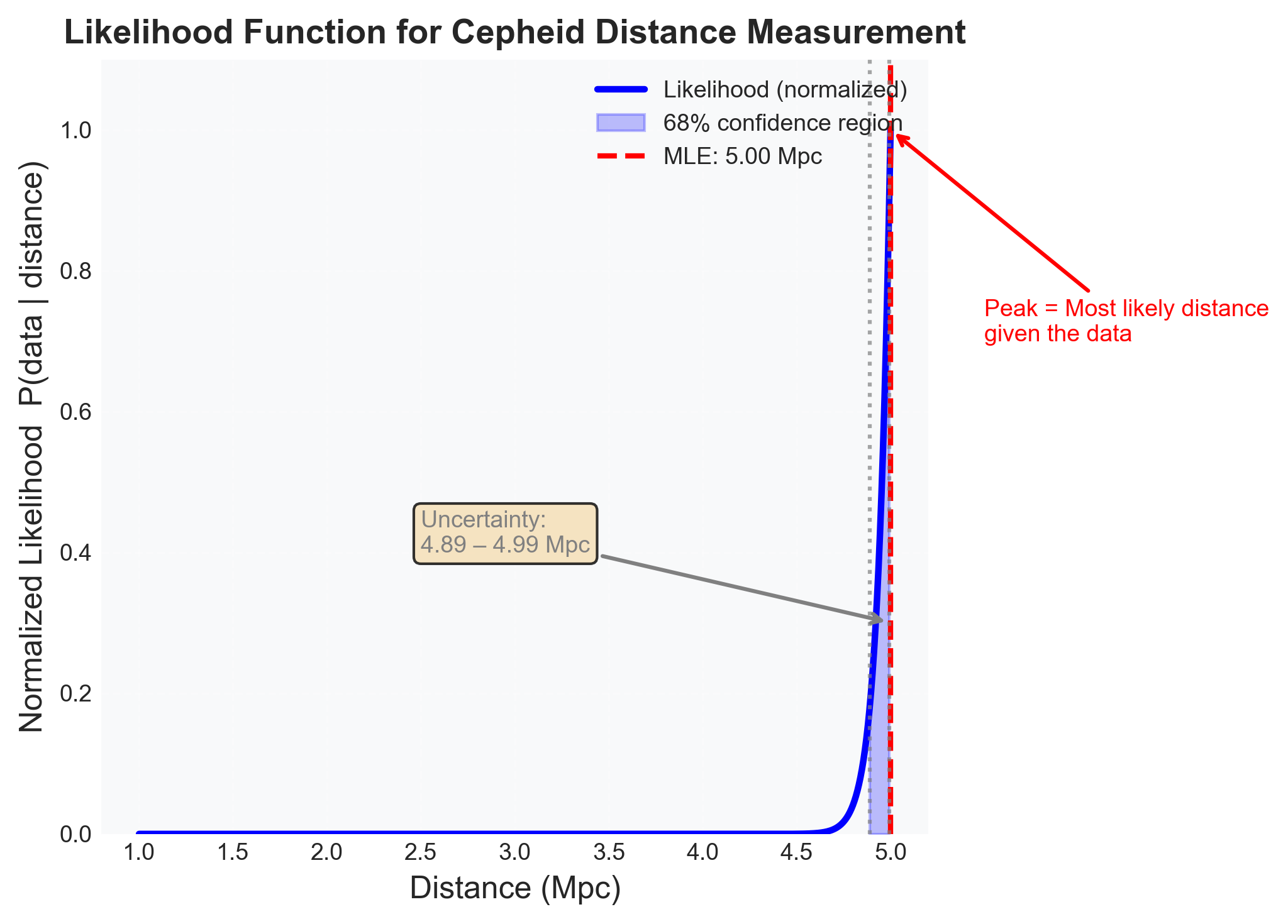
Holding $P$ fixed also means that, within this simplified example,

\[ p(m_{\mathrm{obs}} \mid d, P) = p(m_{\mathrm{obs}} \mid d), \]

because all period uncertainty has been neglected. In a more realistic model, uncertainty in $P$ would be part of the likelihood too.

That gives the observation model

\[ m_{\mathrm{obs}} = m_{\mathrm{model}}(d) + \epsilon, \qquad \epsilon \sim \mathcal{N}(0, \sigma_m^2). \]

Step 3: Likelihood

The corresponding likelihood is

\[ p(m_{\text{obs}} | d) = \mathcal{N}(m_{\text{obs}}; m_{\text{model}}(d), \sigma_m^2) \]

with

$m_{\text{model}}(d) = M_V + 5 \log_{10}(d \times 1000 / 10)$ (d in kpc, distance in pc for the log term)
$\sigma_m = 0.15$ mag (measurement uncertainty)

or, in the exponential form students often implement first,

\[ p(m_{\mathrm{obs}} \mid d) \propto \exp\!\left[ -\frac{\left(m_{\mathrm{obs}} - m_{\mathrm{model}}(d)\right)^2}{2\sigma_m^2} \right]. \]

In log form, which is what the code should evaluate,

\[ \log p(m_{\text{obs}} | d) = -\frac{1}{2} \left[ \frac{(m_{\text{obs}} - m_{\text{model}}(d))^2}{\sigma_m^2} + \log(2\pi\sigma_m^2) \right] \]

Figure 4: **One-dimensional likelihood for a Cepheid-style distance inference.** This is the shape MCMC is trying to explore efficiently once brute-force evaluation becomes too expensive. The key pedagogical point is that the likelihood is already a function you could plot in 1D, inspect, and then later generalize to higher-dimensional posteriors where the same workflow is no longer cheap on a grid.

Step 4: Prior

We now encode a simple scale prior. We will use a prior uniform in log-distance, which corresponds to the density

\[ p(d) \propto \frac{1}{d}. \]

This is a common choice for positive scale parameters because it does not privilege one multiplicative scale over another.

We will actually sample in $\log d$, where the prior is uniform:

\[ p(\log d) = \text{Uniform}[\log(50), \log(10,000)] \]

This corresponds to distances between 50 kpc and 10 Mpc, a reasonable range for extragalactic Cepheids (e.g., in M31, M33, or Local Group galaxies).

Step 5: Posterior

By Bayes’ theorem,

\[ p(d | m_{\text{obs}}) \propto p(m_{\text{obs}} | d) \times p(d) \]

In log form, the quantity we actually hand to the sampler is

\[ \log \pi(d) = \log p(m_{\mathrm{obs}} \mid d) + \log p(d) + C, \]

where the additive constant $C$ does not depend on $d$ and can be dropped.

This is the answer to the practical question “What function do I write?” You write the function that returns $\log p(m_{\mathrm{obs}} \mid d) + \log p(d)$.

Step 6: What Changes in More Than One Parameter?

Real Cepheid inference is rarely this clean. If extinction is also uncertain, then the model becomes

\[ m_{\mathrm{model}}(d, A_V) = M_V + 5 \log_{10}(d / 10~\mathrm{pc}) + A_V. \]

Now distance and extinction trade off against each other: a larger $A_V$ can mimic a larger distance. The posterior becomes a correlated ridge rather than a single narrow bump. That is exactly the kind of geometry MCMC is built for.

In that 2D version, the computational target becomes

\[ \log \pi(d, A_V) = \log p(m_{\mathrm{obs}} \mid d, A_V) + \log p(d) + \log p(A_V) + C. \]

This is the real conceptual bridge from Part 2 to Part 3: the physics and uncertainty model define the posterior, and MCMC supplies the machinery for exploring it when that posterior is no longer something you can exhaustively map on a grid.

Pause and Predict

Before seeing any numerical result, make a scientific prediction:

Roughly what distance should the posterior center on?
Should the posterior be nearly symmetric in $d$, or slightly skewed?
If the proposal scale is tuned reasonably, do you expect the chain to mix quickly in this one-parameter problem?

This matters because MCMC should not feel like a black box. You should have physical expectations before the chain runs.

What the Sampler Should Recover

If you connect the generic Metropolis-Hastings sampler above to this log-likelihood and prior, the chain should recover a posterior centered near $d \approx 323~\text{kpc}$ with a width of a few tens of kiloparsecs.

The important teaching point is not the exact number. It is the structure of the answer:

a central distance estimate near the distance-modulus calculation
a credible interval rather than a single “best” value
a trace plot that reaches stationarity quickly in this simple one-dimensional problem
an autocorrelation time small enough that a modest chain produces a useful effective sample size

For a well-tuned one-dimensional sampler here, an acceptance rate in the rough range of 25% to 50% is plausible, and an autocorrelation time of order $10$ would indicate healthy mixing.

Scientific Interpretation

What changes when we switch from a point estimate to a posterior?

We no longer say only “the star is about 323 kpc away.”
We say “the data support a range of distances, with quantified uncertainty.”
We can propagate that uncertainty forward into later inferences.
We can compare this result consistently with other distance indicators.

That is the real payoff of MCMC. It turns an inverse problem into a defensible uncertainty statement.

Connection to Project 4

This Cepheid example is the local version of what you will do in Project 4 for Type Ia supernovae. The observable changes, the forward model changes, and the parameter space becomes higher dimensional, but the architecture stays the same:

write down the forward model
define the likelihood
encode prior information
sample the posterior
diagnose the chain before trusting the result

The method scales from standard candles in the Local Group to cosmological inference.

Synthesis — The Conceptual Architecture

Where We Are

The complete journey: You’ve traveled from the computational crisis that makes MCMC necessary (Part 1), through the elegant mathematical theory of Markov chains (Part 2), to the ingenious Metropolis-Hastings algorithm (Part 3), learned how to diagnose whether your sampler actually works (Part 4), and applied it all to real astrophysics (Part 5).

Now we zoom out to see the big picture. How do all these pieces fit together? How does MCMC connect to the broader themes of this course — statistical thinking, physical intuition, computational methods? This synthesis reveals the deep unity underlying everything you’ve learned.

You’ve learned a lot. Let’s step back and see the structure of what you now know.

The Four Pillars of MCMC

Conceptual Architecture of MCMC

1. Statistical Foundation (Module 1):

Law of Large Numbers: Sample averages converge to expectations
Central Limit Theorem: Estimation errors scale as $1/\sqrt{N}$
Sampling distributions: Characterize uncertainty via distributions

2. Stochastic Process Theory (Module 5, Part 2):

Markov chains: Memoryless random walks through state space
Stationary distributions: Equilibrium distributions preserved by dynamics
Ergodicity: Time averages equal ensemble averages
Detailed balance: Sufficient condition for stationarity

3. Algorithmic Implementation (Module 5, Part 3):

Proposal distribution $Q$: How to generate candidates
Acceptance probability $\alpha$: When to accept, based on posterior ratio
Metropolis-Hastings: The universal recipe for MCMC sampling

4. Practical Application (Module 5, Parts 4-5):

Diagnostics: Trace plots, R-hat, autocorrelation, ESS
Burn-in: Discarding pre-equilibrium samples
Tuning: Adjusting proposals for efficient exploration
Real inference: From theory to astrophysical discoveries

Each pillar rests on the previous one. You can’t appreciate MCMC diagnostics without understanding Markov chains. You can’t design good samplers without knowing detailed balance. And you can’t trust your results without proper statistical foundations.

One way to summarize the entire lecture is:

Part 1: why posterior computation is hard
Part 2: what kind of stochastic process can solve it
Part 3: how Metropolis-Hastings builds that process
Part 4: how we decide whether to trust the run
Part 5: what scientific interpretation looks like once the machinery works

Universal Patterns Across Modules

One of the profound lessons of this course: The same mathematical structures appear everywhere. Let’s make this explicit:

Concept	Module 1: Statistics	Modules 3: Statistical Mechanics	Module 5: Bayesian Inference
What we’re sampling	Random variables	Microstates in phase space	Parameters in posterior
Target distribution	Population distribution	Boltzmann distribution	Posterior $p(\theta \mid D)$
How we sample	Independent and Identically Distributed (IID) random draws	Molecular dynamics	Markov chain (MCMC)
Why it works	Law of Large Numbers	Ergodic hypothesis	Ergodic theorem
Convergence condition	CLT (independent samples)	Thermal equilibration	Detailed balance
What we compute	Sample statistics	Thermodynamic quantities	Parameter estimates
Time average = ?	Ensemble average (Module 1)	Ensemble average (Module 3)	Expectation under $\pi$ (Module 5)

The profound unity: Whether you’re:

Drawing random samples to estimate a population mean (Module 1)
Simulating molecules reaching thermal equilibrium (Module 3)
Sampling parameters to quantify uncertainty (Module 5)

You’re using the same mathematical structure: stochastic processes converging to equilibrium distributions, with time averages equaling ensemble averages.

This is why physics is so powerful and predictive. The same principles work everywhere, from atoms to stars to probability distributions.

Reflection Question

Before moving on, pause and think:

How is MCMC sampling from $p(\theta \mid D)$ analogous to molecular dynamics sampling from the Boltzmann distribution $p(E) \propto \exp(-E/kT)$?

Write down the correspondence:

Temperature $T$ $\leftrightarrow$ ?
Energy $E$ $\leftrightarrow$ ?
Particle position $x$ $\leftrightarrow$ ?
Boltzmann distribution $\leftrightarrow$ ?

Answer: $T = 1$ (fixed), $E = -\log p(\theta \mid D)$, $x = \theta$, and the Boltzmann distribution $\leftrightarrow$ the posterior.

They’re mathematically identical! Replace energy with negative log-probability, and MCMC is molecular dynamics in parameter space.

From Theory to Practice: Your Toolbox

You now have:

1. Conceptual understanding:

Why MCMC is necessary (curse of dimensionality)
How MCMC works (Markov chains, detailed balance)
When MCMC converges (ergodicity, stationarity)

2. Practical skills:

Implementing Metropolis-Hastings
Tuning proposal distributions
Diagnosing convergence (trace plots, R-hat, ACF)
Interpreting results (corner plots, credible intervals)

3. Scientific applications:

Setting up Bayesian models (likelihood + prior)
Running inference on real data (Cepheids)
Quantifying uncertainty properly

4. Connections:

To Module 1 (sampling, CLT, ergodicity)
To Module 3 (phase space, thermalization, detailed balance)
To Project 4 (Type Ia SNe, cosmological parameters)

This is a complete inference framework you can apply to any scientific problem.

Common Misconceptions About MCMC

Before moving to Project 4, let’s address some frequent misunderstandings that trip up even experienced practitioners:

Misconception 1: “High acceptance rate means good sampling”

Reality: High acceptance (>60%) usually means your proposals are too timid — you’re taking baby steps and exploring slowly. The chain mixes poorly and has high autocorrelation. Conversely, very low acceptance (<15%) means proposals are too aggressive. Optimal acceptance depends on dimension: aim for 20-40% in most cases.

Why it’s tempting: It feels good when proposals are accepted! But acceptance rate is about efficiency, not validity.

Misconception 2: “R-hat < 1.1 guarantees convergence”

Reality: R-hat < 1.1 is necessary but not sufficient for convergence. If your posterior has multiple well-separated modes and each chain gets stuck in one mode, R-hat will look fine but you haven’t converged to the full posterior. You’ve converged to individual modes.

How to catch it: Always visually inspect trace plots and 2D marginal distributions. Look for chains that never overlap. Run chains from diverse starting points spanning the prior range.

Misconception 3: “MCMC samples are independent”

Reality: MCMC samples are correlated. The effective sample size $N_\text{eff} = N/\tau$ accounts for this. If $\tau = 100$, your 10,000 samples carry as much information as 100 independent samples. Always report $N_\text{eff}$, not just $N$.

Practical impact: If you compute credible intervals assuming independence, they’ll be too narrow (overconfident). Use N_eff for uncertainty quantification.

Misconception 4: “Longer chains are always better”

Reality: Running a poorly-tuned chain longer doesn’t fix the problem — it just wastes time. If your proposals are bad, adding more samples doesn’t help. Fix the sampler first (tune step size, use better proposals, add constraints), then run long chains.

The exception: If your chain is well-tuned but exploring a complex posterior, then yes, longer is better. But “longer” means N_eff > 400 per parameter, not just more samples.

Misconception 5: “I can start MCMC anywhere”

Reality: While theory says chains converge from any starting point, starting very far from the typical set (the region of high probability) means long burn-in. Starting outside your prior bounds or at parameter values where the likelihood is undefined will cause immediate failure.

Best practice: Start from reasonable values. For well-specified priors, sample from the prior. For complex problems, run optimization first to find the posterior mode, then start MCMC nearby.

Misconception 6: “Burn-in is waste”

Reality: Burn-in is not waste — it’s how the chain finds the typical set! It’s like a spacecraft’s trajectory correction burns to reach the right orbit. The real waste is keeping burn-in samples and contaminating your posterior estimates.

How much to discard: Be conservative. If in doubt, discard more. Look at trace plots — when do they stabilize?

Misconception 7: “MCMC always works”

Reality: MCMC can fail in many ways:

Multimodal posteriors where chains get trapped in one mode
Extremely high-dimensional problems where mixing is glacially slow
Posteriors with complex geometry (funnel shapes, banana-shaped ridges)
Highly correlated parameters that random walk proposals can’t handle
Likelihood functions with discontinuities or numerical instabilities

Recognition: That’s why diagnostics exist! If R-hat is bad, acceptance is extreme, or chains look weird, don’t trust the results. Fix the sampler or use a different method.

Misconception 8: “The posterior mean is the best parameter estimate”

Reality: Depends on your loss function! The posterior mean minimizes squared-error loss. The posterior median minimizes absolute-error loss. The posterior mode (MAP) minimizes 0-1 loss. Which one you report depends on what you’re trying to do. For asymmetric posteriors, they can differ substantially.

Best practice: Report the full posterior (credible intervals) rather than a single point estimate. Let readers make their own decisions about point estimates.

Looking Ahead: Project 4 and Beyond

What’s Next

In Project 4, you’ll implement everything from this module to measure cosmological parameters from Type Ia supernovae:

Your tasks:

Build the forward model (cosmological distance-redshift relation)
Implement Metropolis-Hastings MCMC
Apply diagnostics (trace plots, R-hat, ACF, corner plots)
Run inference on real SNe data (JLA sample)
Measure $\Omega_m$ and $h$ (the contents of the universe!)
Extend to Hamiltonian Monte Carlo (using your leapfrog integrator from Project 2)

This is the same data and methods that earned the 2011 Nobel Prize in Physics for the discovery of dark energy.

Advanced Topics (Module 5.4 Preview)

After mastering Metropolis-Hastings, you’ll learn:

Hamiltonian Monte Carlo (HMC):

Uses gradient information for efficient exploration
Based on Hamiltonian dynamics (Module 3!)
Much lower autocorrelation than random walk
The leapfrog integrator from Project 2 is exactly what HMC uses

Affine-invariant ensemble samplers (like emcee):

Multiple “walkers” evolve together
Self-tuning, no manual proposal tuning needed
Handles strong correlations automatically

No-U-Turn Sampler (NUTS):

Adaptive HMC that automatically tunes step size and trajectory length
The algorithm behind Stan and PyMC
State of the art for general-purpose MCMC

But these are all variations on the core principles you learned here. Metropolis-Hastings is the foundation.

Where is MCMC Heading? The Frontier of Computational Inference

MCMC is not a settled field — it’s actively evolving. Here are some exciting research directions that may transform how we do inference in the next decade:

Neural network-assisted MCMC: Recent work uses machine learning to learn optimal proposal distributions from data. Instead of hand-tuning proposals, train a neural network to predict good proposals based on the posterior landscape. Early results show dramatic speedups for complex problems. This combines classical statistics with modern deep learning.

Adaptive and self-tuning methods: Modern samplers can adapt their behavior during sampling without violating detailed balance (which traditional theory said was impossible!). Methods like adaptive Metropolis (Haario et al. 2001) and delayed rejection algorithms show that we can be smarter about exploration while maintaining theoretical guarantees.

Non-reversible MCMC: Traditional MCMC satisfies detailed balance (microscopic reversibility). But what if we intentionally break reversibility to explore faster? Non-reversible Langevin samplers and lifted particle filters can have much lower autocorrelation than reversible methods. This is cutting-edge research connecting to non-equilibrium statistical mechanics.

Variational inference and hybrid methods: Not everything requires sampling. Variational methods approximate posteriors with simpler distributions (like Gaussians) by optimization rather than sampling. Modern hybrid approaches combine MCMC’s accuracy with variational inference’s speed. The future may be algorithms that switch between sampling and optimization adaptively.

Quantum MCMC: As quantum computers mature, researchers are developing quantum algorithms for Bayesian inference. Quantum walks could explore posterior landscapes exponentially faster than classical MCMC — though practical implementations are years away.

Amortized inference: Instead of running MCMC separately for each dataset, train a model once that can instantly produce posteriors for new data. This “simulation-based inference” approach (also called likelihood-free inference or neural posterior estimation) is revolutionizing fields where likelihood evaluation is expensive.

The common thread: All these advances build on the foundations you learned — Markov chains, stationarity, convergence theory. Understanding Metropolis-Hastings deeply prepares you to understand and contribute to these cutting-edge methods. The principles don’t change; the implementations get ever more sophisticated.

MCMC has come a long way from simulating nuclear reactions on MANIAC I in 1953. Where will it go next? Perhaps you’ll help decide.

The Professional Path

After building MCMC from scratch, you’ll be able to use professional tools intelligently:

emcee (Python): Affine-invariant ensemble sampler
PyMC (Python): Full Bayesian modeling framework with HMC/NUTS
Stan (C++): Gold-standard Bayesian inference (autodiff, NUTS)
JAX/numpyro (Python): HMC with Just-In-Time (JIT) compilation and GPU acceleration

You won’t be a black-box user clicking buttons. You’ll understand:

Why these tools work (detailed balance, ergodicity)
How to diagnose problems (R-hat, trace plots, divergences)
When methods fail (multimodal posteriors, stiff likelihoods)
What the algorithms are actually doing under the hood

That’s the glass-box philosophy in action.

Congratulations! You’ve learned one of the most important computational techniques in modern science. MCMC underpins:

Bayesian inference across all sciences
Machine learning (Bayesian neural networks, variational inference)
Computational physics (lattice QCD, molecular dynamics)
Statistics (everywhere!)

More importantly, you’ve seen how measurement, probability, physics, and computation all connect into a unified framework for learning from data.

Now go build your inference engine. The universe is waiting to be measured.

Learning Outcomes

Roadmap: Where We’re Going

Part 1: The Computational Crisis — Why We Need MCMC

The Posterior is a Distribution, Not a Number

A Complete Inference Pipeline You Could Reconstruct

The Curse of Dimensionality

What About Optimization? Just Find the Peak

What Inference Actually Requires

The Monte Carlo Solution: Sample, Don’t Integrate

Part 2: Markov Chains — The Mathematical Foundation

The Core Idea: Build a Stochastic Process

Markov Chains: Formal Definition

Transition Kernels

Stationarity: The Distribution Must Be Preserved

Ergodicity: The Chain Must Explore Everywhere

Detailed Balance: A Sufficient Condition for Stationarity

Part 3: The Metropolis-Hastings Algorithm

The Construction: Proposal + Accept/Reject

Deriving the Acceptance Probability

Proposal Distributions: Symmetric vs. Asymmetric

Tuning the Proposal: The Art of Step Size

From Likelihood to Log-Posterior Code

Minimal Sampler Skeleton

What About the Normalization Constant?

Part 4: Practical Diagnostics — Has Your Chain Converged?

Visual Diagnostic: Trace Plots

Quantitative Diagnostic 1: Autocorrelation Function

Quantitative Diagnostic 2: Gelman-Rubin Statistic

Burn-In: How Much to Discard?

Putting It All Together: A Convergence Checklist

Failure Modes to Watch For

Part 5: Real Example — Cepheid Variable Distance

The Science: Cepheids as Standard Candles

The Problem: Inferring Distance from Photometry

Step 1: Forward Model

Step 2: Noise Model and Likelihood Assumptions

Step 3: Likelihood

Step 4: Prior

Step 5: Posterior

Step 6: What Changes in More Than One Parameter?

Pause and Predict

What the Sampler Should Recover

Scientific Interpretation

Synthesis — The Conceptual Architecture

The Four Pillars of MCMC

Universal Patterns Across Modules

From Theory to Practice: Your Toolbox

Common Misconceptions About MCMC

Looking Ahead: Project 4 and Beyond

What’s Next

Advanced Topics (Module 5.4 Preview)

Where is MCMC Heading? The Frontier of Computational Inference

The Professional Path

Self-Assessment Rubric

Level 1: Conceptual Understanding

Level 2: Mathematical Foundations

Level 3: Implementation Skills

Level 4: Diagnostic Expertise

Level 5: Scientific Application

Level 6: Connections and Transfer