Part II: Mathematical Foundations of Radiative Transfer
From Intuition to Equations | Statistical Thinking Module 4 | COMP 536
“The book of nature is written in the language of mathematics.” – Galileo Galilei
Learning Objectives
By the end of Part II, you will be able to:
- Define specific intensity \(I_\nu(\vec{r}, \hat{n}, t)\) and explain why it’s the fundamental quantity for radiation
- Calculate moments of intensity to derive flux, energy density, and radiation pressure
- Derive the radiative transfer equation from conservation principles
- Incorporate scattering into the radiative transfer framework
- Solve the RTE for simple cases (pure absorption, uniform medium)
- Apply the formal solution to compute emergent intensities
- Connect the mathematical framework to physical observables
This part transforms Part I’s physical intuition into precise mathematical language through three interconnected developments:
Section 2.1: Statistical Description of Radiation Fields You’ll learn why specific intensity is THE fundamental quantity — all observables (flux, pressure, energy density) emerge as its moments. This parallels how thermodynamics emerges from particle distributions.
Section 2.2: The Radiative Transfer Equation You’ll derive the master equation governing radiation propagation. Just as Newton’s laws describe particle motion, the RTE describes how photon intensities change along rays when radiation interacts with matter.
Section 2.3: Scattering and Complete Transport You’ll extend the framework to include scattering, seeing how photons redistribute rather than simply disappear. This completes the mathematical foundation needed for realistic radiative transfer.
The Big Picture: These equations aren’t abstract — they’re the tools that let us decode what we observe. Every astronomical spectrum, every dusty image, every radiative transfer calculation rests on this mathematical foundation.
From Physical Pictures to Mathematical Precision
In Part I, we built intuition about how photons carry information across the cosmos, how dust transforms their journey, and why different wavelengths reveal different physics. Now we elevate that intuition to mathematical precision. The equations we’re about to develop aren’t academic exercises — they’re the foundation of every radiative transfer code, every atmospheric model, every stellar atmosphere calculation. When JWST analyzes an exoplanet atmosphere or when you implement Monte Carlo transport in Project 3, these are the equations at work.
The profound insight is that all radiation phenomena — from stellar spectra to dust extinction to greenhouse effects — follow from a single master equation: the radiative transfer equation (RTE). Just as Newton’s second law \(F = ma\) governs all classical mechanics, the RTE governs all radiation propagation and its interaction with matter. Master this equation and you hold the key to understanding how light moves through the universe.
2.1 Statistical Description of Radiation Fields
Priority: 🔴 Essential.
To describe radiation mathematically, we need a quantity that captures everything about the light field at any point. This quantity must encode not just “how much” light but also its color (frequency), direction of travel, position, and how it changes with time. The genius insight of radiative transfer theory is that one quantity — specific intensity — contains all this information, and everything else we measure derives from it.
Throughout Part II, we use frequency-based notation:
- \(I_\nu\) = specific intensity per unit frequency [erg cm⁻² s⁻¹ Hz⁻¹ sr⁻¹]
- \(\kappa_\nu\) = opacity at frequency ν
- \(S_\nu\) = source function at frequency ν
To convert to wavelength units:
\[I_\lambda = I_\nu \left|\frac{d\nu}{d\lambda}\right| = I_\nu \frac{c}{\lambda^2}\]
The factor \(c/\lambda^2\) comes from \(\nu = c/\lambda\), so \(|d\nu/d\lambda| = c/\lambda^2\).
Key point: The integral of intensity over all frequencies equals the integral over all wavelengths:
\[\int_0^\infty I_\nu d\nu = \int_0^\infty I_\lambda d\lambda\]
We use frequency notation because:
- Planck’s law is simpler in frequency
- Photon energies are \(E = h\nu\)
- Atomic transitions have fixed frequencies
Vector notation: We use \(\vec{r}\) for position vectors and \(\hat{n}\) for unit direction vectors throughout.
2.1.1 The Fundamental Quantity: Specific Intensity
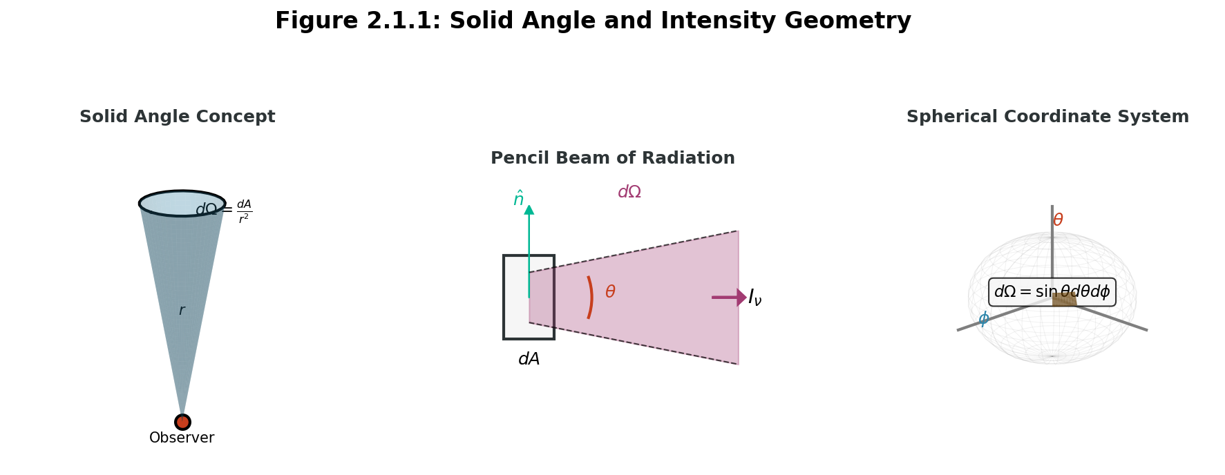
Solid Angle \(\Omega\) A 2D angle in 3D space, measuring the size of an object as seen from a point. Unit: steradian (sr) = rad\(^2\). Full sphere = 4π sr.
Imagine standing at a point in space with a tiny detector (area \(dA\)) that can measure light (\(dE\)) coming from a specific direction \(\vec{r}\) within a small solid angle \((d\Omega)\), at a specific frequency within a narrow band \((\nu + d\nu)\), during a brief time interval \((dt)\). The specific intensity is what this idealized detector measures:
\[ \boxed{I_\nu(\vec{r}, \hat{n}, t) = \frac{dE}{dA \, dt \, d\nu \, d\Omega}} \]
Each element in this equation has precise physical meaning. Since we’re dealing with differential quantities, we’re measuring energy flow within small ranges, not at exact single values.
Components of Specific Intensity:
- \(dE\): Energy passing through the detector [erg in CGS]
- \(dA\): Area of detector perpendicular to beam [cm²]
- \(dt\): Time interval of measurement [s]
- \(d\nu\): Frequency bandwidth [Hz]
- \(d\Omega\): Solid angle subtended by source [steradian]
Important: The area \(dA\) is measured perpendicular to the direction \(\hat{n}\) of the beam. If the detector surface is tilted at angle \(\theta\) to the beam, the effective area is \(dA_{\text{eff}} = dA \cos\theta\).
The Full Symbol Breakdown:
- \(I_\nu\): The intensity at frequency \(\nu\)
- \(\vec{r}\): Position vector (where we’re measuring)
- \(\hat{n}\): Unit vector pointing toward the light source
- \(t\): Time of measurement
Units: [erg cm⁻² s⁻¹ Hz⁻¹ sr⁻¹] in CGS
This five-dimensional differential makes specific intensity seem complex, but it’s the price we pay for completeness. We need all this information to fully characterize the radiation field.
Why Specific Intensity is Fundamental
Specific intensity has three crucial properties that make it the fundamental quantity:
- It’s conserved along rays in vacuum: As light travels through empty space, \(I_\nu\) remains constant along the ray
- All observables are its moments: Flux, energy density, and radiation pressure emerge from integrating \(I_\nu\)
- It directly enters the transfer equation: The RTE describes how \(I_\nu\) changes due to matter
Let’s explore each property with explicit calculations.
2.1.2 From Intensity to Observable Quantities: The Power of Moments
All measurable radiation quantities emerge as moments of the specific intensity. This is analogous to how:
- Pressure and temperature emerge from molecular velocity distributions in Module 1.
- Fluid properties emerge from particle distributions in Module 2.
- Stellar velocity distributions emerge from gravitational interactions in Module 3.
 {#fig:solid_angle width=“100%” fig-align=“center”}
Let’s calculate how flux emerges from specific intensity through angular integration. Consider a star with uniform surface brightness (limb-darkened stars come later).
Setup: Star has intensity \(I_0\) across its visible disk, zero elsewhere.
Step 1: Define the geometry.
- Observer at distance \(d\) from star of radius \(R\)
- Star subtends solid angle \(\Omega_* = \pi(R/d)^2\) for \(d \gg R\)
- Use spherical coordinates: \((\theta, \phi)\) centered on line of sight
Step 2: Set up the flux integral. The flux \(F_\nu\) through a surface is the integral of intensity over solid angle, weighted by \(\cos\theta\):
\[F_\nu = \int I_\nu \cos\theta \, d\Omega\]
The \(\cos\theta\) factor accounts for the projection of the surface normal onto the line of sight.
Step 3: Express the solid angle element explicitly.
In spherical coordinates, the solid angle element is: \[d\Omega = \sin\theta \, d\theta \, d\phi\]
This is crucial! The \(\sin\theta\) comes from the Jacobian of the spherical coordinate transformation.
Important note on units: Solid angle has units of steradians (sr), where 1 sr = 1 radian². However, since radians are dimensionless (angle = arc length/radius), steradians are often treated as dimensionless too. This is why we frequently don’t write “sr” explicitly, but it’s there! This becomes important when understanding why the mean intensity \(J_\nu = \frac{1}{4\pi}\int I_\nu d\Omega\) has the same units as \(I_\nu\) - the 1/4π has implicit units of sr⁻¹ that cancel with the sr from \(d\Omega\).
So our flux integral becomes: \[F_\nu = \int_0^{2\pi} d\phi \int_0^{\theta_*} I_0 \cos\theta \sin\theta \, d\theta\]
Step 4: Evaluate the integrals.
- \(\phi\) integral: gives \(2\pi\)
- \(\theta\) integral: Use substitution \(u = \cos\theta\), \(du = -\sin\theta d\theta\)
When \(\theta = 0\): \(u = 1\) When \(\theta = \theta_*\): \(u = \cos\theta_*\)
\[F_\nu = 2\pi I_0 \int_{\cos\theta_*}^{1} u \, du = 2\pi I_0 \left[\frac{u^2}{2}\right]_{\cos\theta_*}^{1}\]
\[F_\nu = \pi I_0 (1 - \cos^2\theta_*) \approx \pi I_0 \theta_*^2 = \pi I_0 \left(\frac{R}{d}\right)^2\]
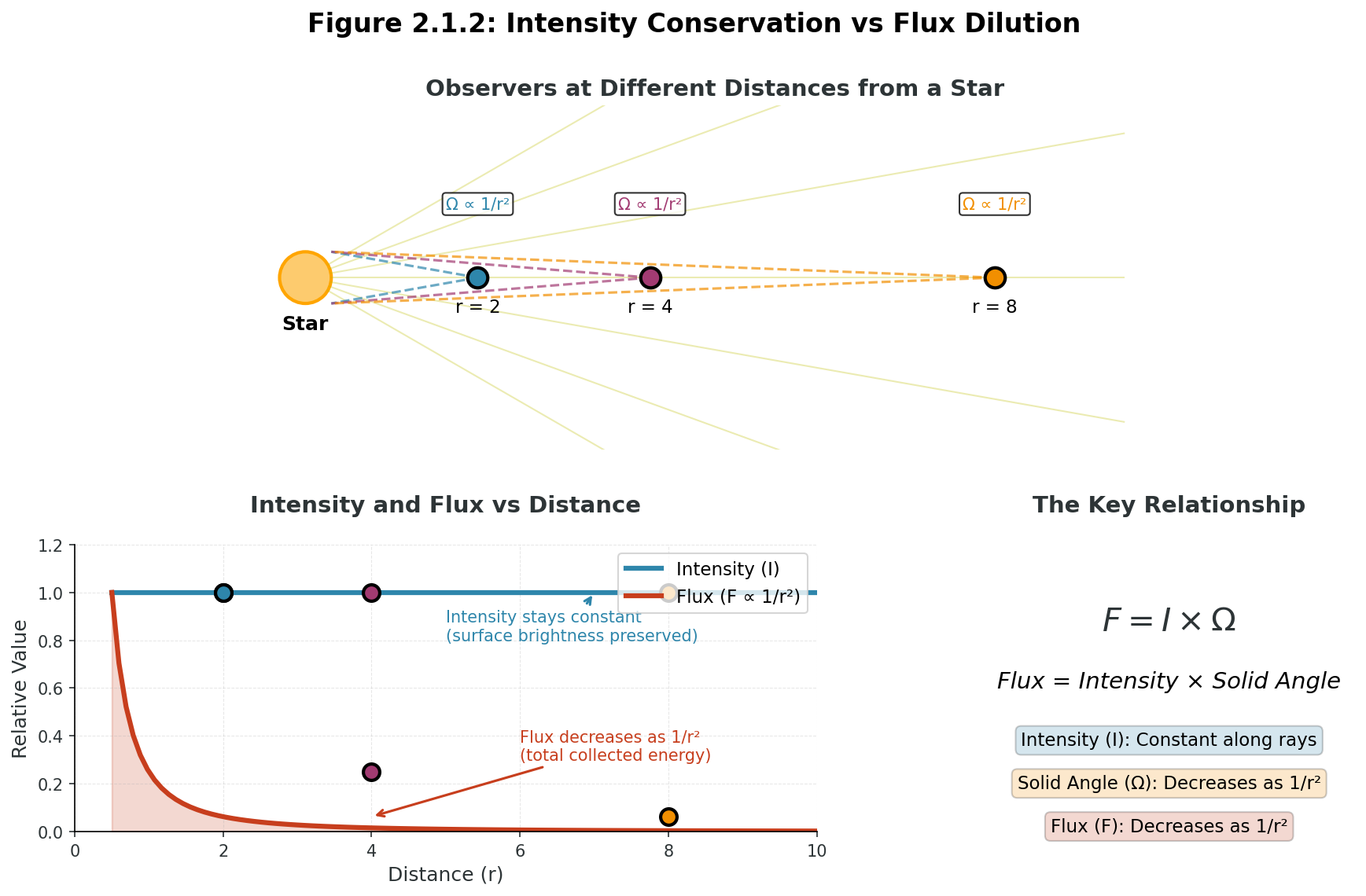
Key Result: Flux decreases as \(1/d^2\) (inverse square law) while intensity \(I_0\) stays constant!
The Complete Set of Moments
0th Moment - Energy Density: \[u_\nu = \frac{1}{c} \int_{4\pi} I_\nu \, d\Omega = \frac{4\pi}{c} J_\nu\]
where \(J_\nu = \frac{1}{4\pi}\int I_\nu d\Omega\) is the mean intensity.
1st Moment - Flux: \[F_\nu = \int_{4\pi} I_\nu \cos\theta \, d\Omega\]
2nd Moment - Radiation Pressure: \[P_\nu = \frac{1}{c} \int_{4\pi} I_\nu \cos^2\theta \, d\Omega\]
For isotropic radiation: \(P = \frac{1}{3}u\) (factor of 1/3 from angular averaging of \(\cos^2\theta\)).
Consider a distant star cluster like NGC 3603. Even though billions of photons with complex angular distributions hit your telescope, you record just one number per wavelength bin - the flux. Yet from this simple measurement, combined with spectroscopy, we can determine:
- The cluster’s total luminosity (from flux and distance)
- Its temperature distribution (from the spectrum shape)
- The dust column density (from reddening)
- Even dynamical information (from line widths)
Question to ponder: If we could measure the full specific intensity \(I_\nu(\hat{n})\) for every direction, what additional information would we gain? Think about this before reading on…
Answer: We could create a full 3D map of the dust distribution! Different sight lines through the cloud would show different extinction. This is why integral field spectroscopy is so powerful - it gives us spatial and spectral information simultaneously.
Let’s make this concrete with NGC 3603 observations:
What we measure:
- Flux in V-band: \(F_V = 2 \times 10^{-13}\) erg/cm²/s/Å at Earth
- Angular size: 10 arcmin = 0.003 radians
Deriving the intensity: The cluster subtends solid angle \(\Omega = \pi \theta^2 = \pi (0.003)^2 = 2.8 \times 10^{-5}\) sr
If we assume uniform surface brightness: \[I_V = \frac{F_V}{\Omega} = \frac{2 \times 10^{-13}}{2.8 \times 10^{-5}} = 7 \times 10^{-9} \text{ erg/cm²/s/Å/sr}\]
Energy density at Earth: \[u_V = \frac{4\pi I_V}{c} = \frac{4\pi \times 7 \times 10^{-9}}{3 \times 10^{10}} = 3 \times 10^{-18} \text{ erg/cm³/Å}\]
Radiation pressure: \[P_V = \frac{u_V}{3} = 10^{-18} \text{ dyne/cm²/Å}\]
This is 15 orders of magnitude below atmospheric pressure - radiation pressure from NGC 3603 is utterly negligible at Earth! But near the massive stars themselves, radiation pressure dominates and drives powerful stellar winds.
Students often confuse intensity and flux. Here’s the key distinction:
Intensity (\(I_\nu\)):
- Power per unit area, per frequency, per solid angle
- Conserved along rays in vacuum
- Doesn’t decrease with distance
- What determines surface brightness
Flux (\(F_\nu\)):
- Power per unit area, per frequency (integrated over angles)
- Decreases as \(1/r^2\) with distance
- What we measure with detectors
- Energy actually collected by telescope
Analogy: Intensity is like the brightness of a light bulb’s surface. Flux is like how much light hits your eye. As you move away, the bulb looks smaller (less solid angle) but equally bright (same intensity), while less total light reaches you (flux decreases).
 {#fig:intensity_vs_flux width=“100%” fig-align=“center”}
Here’s a profound fact: the surface brightness (intensity) of an extended object like a galaxy doesn’t change with distance! A galaxy at \(z=0.1\) has the same surface brightness as at would at \(z=1\) (ignoring cosmological effects).
Question: If surface brightness doesn’t change with distance, why do distant galaxies appear fainter?
Answer: They subtend a smaller solid angle! The total flux (brightness) equals intensity times solid angle: $F = I \(\times\) Ω$. As distance increases, \(Ω\) decreases as \(1/r²\), so \(F\) decreases as \(1/r²\), but \(I\) stays constant. This is why we can measure properties of distant galaxies - their surface brightness profiles are preserved!
This principle is so fundamental that it’s used as a cosmological test. In an expanding universe, surface brightness actually dims as \((1+z)⁴\) due to universal expansion and redshift effects - a key test of cosmological models!
You might wonder why we need such a complex quantity as specific intensity. Here’s why it’s essential:
- Completeness: It contains ALL information about the radiation field — position, direction, frequency, and time dependence
- Conservation: Unlike flux, it’s conserved along rays in vacuum, making it trackable
- Foundation: Every observable (what telescopes measure) derives from moments of specific intensity
- Universality: The same quantity describes radiation in stars, galaxies, dust clouds, and even the CMB
Without specific intensity, we couldn’t write the radiative transfer equation, and without the RTE, we couldn’t understand how light propagates through the universe. This single quantity unlocks everything from stellar atmospheres to cosmological radiative transfer.
The payoff: Once you master manipulating specific intensity, you can model any radiation phenomenon in astrophysics — from the greenhouse effect on Venus to light echoes from supernovae to the Sunyaev-Zel’dovich effect in galaxy clusters.
2.2 The Radiative Transfer Equation
Priority: 🔴 Essential.
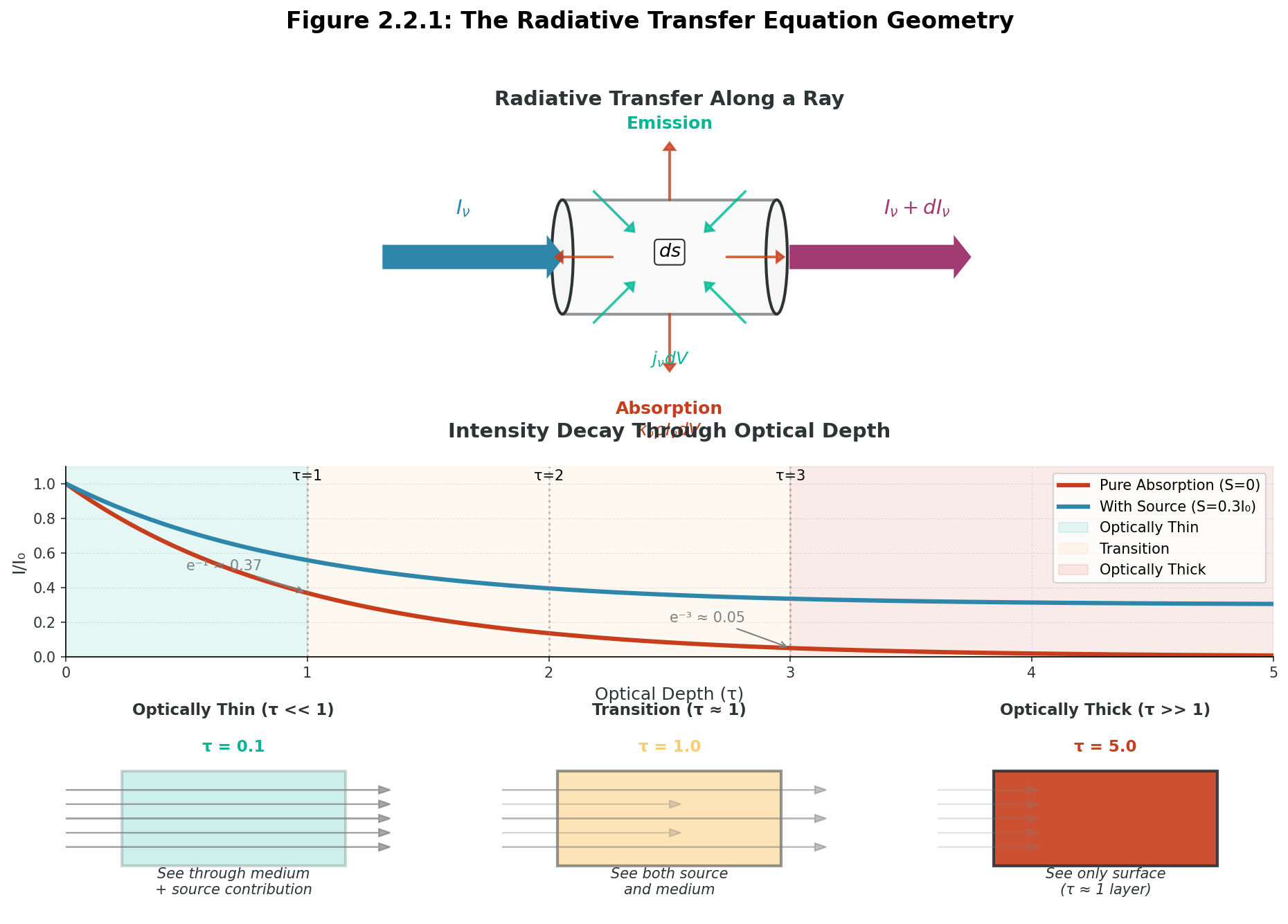
Now we derive the master equation that governs how radiation propagates through matter. The radiative transfer equation emerges from a simple principle: energy conservation along a ray. What goes in must equal what comes out plus what’s created minus what’s destroyed.
Deriving the RTE from First Principles
Consider a cylinder of cross-section \(dA\) and length \(ds\) along a ray direction \(\hat{n}\). Track the energy budget:
Before diving into the RTE, let’s understand why optical depth \(\tau\) is the natural variable for radiative transfer.
Physical Meaning: Optical depth counts “mean free paths”
- \(\tau = 1\): One average interaction length
- \(\tau \ll 1\): Optically thin (transparent)
- \(\tau \gg 1\): Optically thick (opaque)
Why it simplifies math: The RTE in physical units: \[\frac{dI_\nu}{ds} = -\kappa_\nu \rho I_\nu + j_\nu\]
becomes in optical depth: \[\frac{dI_\nu}{d\tau_\nu} = -I_\nu + S_\nu\]
Much cleaner! The absorption coefficient and density combine into one dimensionless variable.
Energy removed (absorption + scattering out): \[dE_{\text{out}} = \kappa_\nu \rho I_\nu \, dA \, ds \, dt \, d\nu \, d\Omega\]
Energy added (emission + scattering in): \[dE_{\text{in}} = j_\nu \, dA \, ds \, dt \, d\nu \, d\Omega\]
where:
- \(\kappa_\nu\) = opacity [cm²/g] - cross-section per unit mass
- \(\rho\) = density [g/cm³]
- \(j_\nu\) = emission coefficient [erg/cm³/s/Hz/sr]
Conservation requires: Change in intensity = Sources - Sinks
\[\frac{dI_\nu}{ds} = -\kappa_\nu \rho I_\nu + j_\nu\]
This is the Radiative Transfer Equation in its most general form!
Always verify your equations are dimensionally consistent. For the RTE:
\[\frac{dI_\nu}{ds} = -\kappa_\nu \rho I_\nu + j_\nu\]
Left side: \(\frac{[I_\nu]}{[s]} = \frac{\text{erg cm}^{-2} \text{s}^{-1} \text{Hz}^{-1} \text{sr}^{-1}}{\text{cm}} = \text{erg cm}^{-3} \text{s}^{-1} \text{Hz}^{-1} \text{sr}^{-1}\)
Right side (absorption): \([\kappa][\rho][I_\nu] = \frac{\text{cm}^2}{\text{g}} \times \frac{\text{g}}{\text{cm}^3} \times \text{erg cm}^{-2} \text{s}^{-1} \text{Hz}^{-1} \text{sr}^{-1}\) \(= \text{erg cm}^{-3} \text{s}^{-1} \text{Hz}^{-1} \text{sr}^{-1}\) ✓
Right side (emission): \([j_\nu] = \text{erg cm}^{-3} \text{s}^{-1} \text{Hz}^{-1} \text{sr}^{-1}\) ✓
Dimensions match! This confirms our equation is physically consistent.
Why this matters: A dimension mismatch immediately reveals an error. If your RTE doesn’t balance dimensionally, you’ve made a mistake in the physics or mathematics.
Understanding the Source Function
Before we proceed, let’s understand the physical meaning of the source function \(S_\nu\). We define:
\[S_\nu = \frac{j_\nu}{\kappa_\nu \rho}\]
Why is this ratio meaningful? The source function represents the intensity that would result if emission and absorption were in perfect balance at that location. To see this, consider what happens when the intensity equals the source function:
\[\frac{dI_\nu}{ds} = -\kappa_\nu \rho I_\nu + j_\nu = -\kappa_\nu \rho I_\nu + \kappa_\nu \rho S_\nu\]
If \(I_\nu = S_\nu\), then: \[\frac{dI_\nu}{ds} = -\kappa_\nu \rho S_\nu + \kappa_\nu \rho S_\nu = 0\]
The intensity doesn’t change! This is radiative equilibrium - emission exactly balances absorption. Just as in Module 2 where hydrostatic equilibrium meant pressure gradient balanced gravity (\(\frac{dP}{dr} = -\frac{GM_r\rho}{r^2}\)), here the radiation field has found its balance point.
Physical Interpretation: The source function tells us what intensity the medium “wants” to create. If \(I_\nu < S_\nu\), the medium adds photons (net emission). If \(I_\nu > S_\nu\), the medium removes photons (net absorption). The radiation field always evolves toward the local source function.
In Local Thermodynamic Equilibrium (LTE), the source function equals the Planck function: \[S_\nu = B_\nu(T) = \frac{2h\nu^3}{c^2} \frac{1}{e^{h\nu/kT} - 1}\]
This occurs when collisions dominate over radiative processes, maintaining a Maxwellian velocity distribution. The medium emits as a blackbody at the local temperature.
Throughout this course, we encounter different types of equilibrium, but they all share the same fundamental principle: competing effects balance to create stability. Here’s how radiative equilibrium connects to what you’ve learned:
Hydrostatic Equilibrium (Module 2 - Stellar Structure): \[\frac{dP}{dr} = -\frac{GM_r\rho}{r^2} \quad \text{(pressure gradient balances gravity)}\]
- Outward pressure force exactly cancels inward gravitational force
- When violated: star expands (pressure wins) or contracts (gravity wins)
- Timescale to restore: sound crossing time (~hours for the Sun)
Radiative Equilibrium (Module 4 - This equation): \[\frac{dI_\nu}{ds} = 0 \text{ when } I_\nu = S_\nu \quad \text{(emission balances absorption)}\]
- Photons added by emission exactly equal photons removed by absorption
- When violated: intensity grows (emission wins) or decays (absorption wins)
- Timescale to restore: photon mean free path time (~microseconds in stellar interior)
Virial Equilibrium (Module 3 - Stellar Systems): \[2K + W = 0 \quad \text{(kinetic energy balances potential energy)}\]
- Kinetic energy (dispersive) balances half the binding energy (attractive)
- When violated: system expands (too hot) or collapses (too cold)
- Timescale to restore: dynamical time (~millions of years for star clusters)
The Deep Pattern: Nature abhors imbalance. When any system is pushed away from equilibrium, restoring forces arise:
- Too much pressure? Expand to reduce it.
- Too much absorption? Intensity decreases until emission can compete.
- Too much kinetic energy? System expands, converting kinetic to potential.
Why the factor of 2 in virial but not others? It comes from the \(1/r\) nature of gravity! The specific mathematical form of each equilibrium depends on the underlying physics, but the principle is universal.
Computational Insight: In your simulations, these equilibria become diagnostics:
- Project 2 (N-body): Check \(|2K + W|/|W| < 0.01\) for equilibrium
- Project 3 (Radiative Transfer): Verify \(I \to S\) in optically thick regions
- All projects: Energy conservation tells you if physics is violated
These aren’t separate concepts — they’re different manifestations of nature’s tendency toward balance!
The radiative transfer equation emerged from multiple influential astrophysicists working on different problems, eventually realizing they were all solving the same fundamental equation:
Karl Schwarzschild (1906): While working on stellar atmospheres, developed the concept of radiative equilibrium. Yes, the same Schwarzschild who gave us black holes! He showed that stars transport energy through radiation in a calculable way.
Arthur Schuster (1905): Introduced the concepts of emission and absorption coefficients while studying fog and planetary atmospheres. His work laid the foundation for understanding scattering.
Edward Arthur Milne (1921): Extended the theory to stellar interiors and developed the concept of optical depth. His work connected thermodynamics to radiation transport.
Subrahmanyan Chandrasekhar (1950s): Provided the complete mathematical framework in his monumental book “Radiative Transfer.” He solved the RTE for various geometries and scattering scenarios, work that helped earn him the Nobel Prize. His solutions for polarized radiation transport are still used today!
The Revolution: Before this unification, each field had its own equations - meteorologists for Earth’s atmosphere, astronomers for stars, engineers for furnaces. The recognition that one equation governed all radiation transport was as profound as Newton realizing the same gravity that drops apples also moves planets!
Today, the same RTE is solved in:
- Climate models (greenhouse effect)
- Medical imaging (X-ray and MRI)
- Computer graphics (realistic rendering)
- Astrophysics (from stars to cosmology)
- Nuclear reactor design (neutron transport)
The universality Chandrasekhar demonstrated continues to enable new applications across science and technology.
Optical Depth: The Natural Variable
Define the optical depth differential: \[d\tau_\nu = \kappa_\nu \rho \, ds\]
This dimensionless quantity measures the “optical thickness” of the material. Integrating:
\[\tau_\nu(s) = \int_0^s \kappa_\nu(s') \rho(s') \, ds'\]
The RTE becomes beautifully simple: \[\boxed{\frac{dI_\nu}{d\tau_\nu} = -I_\nu + S_\nu}\]
The mean free path \(\ell = 1/(n\sigma)\) is a statistical quantity. Individual photons travel different distances before interacting:
The Poisson Process: Photon interactions follow Poisson statistics. The probability of traveling distance \(s\) without interaction is: \[P(s) = e^{-s/\ell} = e^{-\tau}\]
where \(\tau = s/\ell\) is the optical depth.
This is why we sample path lengths using \(s = -\ell \ln(\xi)\) in Monte Carlo, where \(\xi\) is a uniform random number [0,1]!
Key insight: When we say \(\tau = 1\), we mean on average 63% of photons have interacted (1 - e⁻¹ ≈ 0.63), not that every photon interacts at exactly this depth.
Connection to Module 1: This exponential distribution is the same one used for radioactive decay — both are memoryless processes where the probability of an event doesn’t depend on how long you’ve been waiting.
Optical depth relates directly to column density — what astronomers actually measure:
\[\tau = \int n \sigma \, ds = \sigma N\]
where \(N = \int n \, ds\) is the column density [particles/cm²].
For standard Milky Way ISM dust: \[\tau_V \approx 1.8 \times 10^{-21} N_H\]
where \(N_H\) is the hydrogen column density in cm⁻². This relationship varies significantly in other environments (e.g., different in the Magellanic Clouds, starburst galaxies).
Typical values:
- Diffuse ISM: \(N_H \sim 10^{20}\) cm⁻² \(\to\) \(\tau_V \sim 0.18\) (mostly transparent)
- Molecular cloud edge: \(N_H \sim 10^{21}\) cm⁻² \(\to\) \(\tau_V \sim 1.8\) (transition to opaque)
- Dark cloud core: \(N_H \sim 10^{22}\) cm⁻² \(\to\) \(\tau_V \sim 18\) (very opaque)
- Galactic center: \(N_H \sim 10^{23}\) cm⁻² \(\to\) \(\tau_V \sim 180\) (completely opaque in optical)
This is why we need infrared and radio observations to penetrate dense regions!
The RTE is actually a Boltzmann equation for photons! Compare:
Boltzmann equation (for particles, Modules 1 & 2): \[\frac{\partial f}{\partial t} + \vec{v} \cdot \nabla f + \vec{F} \cdot \nabla_v f = \left(\frac{\partial f}{\partial t}\right)_{\text{coll}}\]
Radiative Transfer equation (for photons): \[\frac{1}{c}\frac{\partial I_\nu}{\partial t} + \hat{n} \cdot \nabla I_\nu = -\kappa_\nu \rho I_\nu + j_\nu\]
The Deep Connection:
- Distribution function: \(f(\vec{r}, \vec{v}, t)\) for particles is analogous to \(I_\nu(\vec{r}, \hat{n}, t)\) for photons
- Streaming: \(\vec{v} \cdot \nabla f\) (particles) is analogous to \(c \, \hat{n} \cdot \nabla I_\nu\) (photons)
- Forces: Missing for photons in flat spacetime
- Collisions: Particle scattering is analogous to photon absorption/emission
Same mathematical structure, different physics!
Simple Solutions of the RTE
Let’s solve the RTE for two fundamental cases that build intuition:
Case 1: Pure Absorption (No Emission).
With \(S_\nu = 0\) (no emission), the RTE becomes:
\[\frac{dI_\nu}{d\tau_\nu} = -I_\nu\]
This has the simple solution:
\[I_\nu(\tau) = I_\nu(0) e^{-\tau}\]
This is Beer’s law from Part I! Intensity decreases exponentially with optical depth.
The exponential function \(e^{-\tau}\) appears constantly in radiative transfer. Key properties:
Values to remember:
- \(e^0 = 1\) (no extinction)
- \(e^{-1} \approx 0.368\) (about 37% transmission at \(\tau = 1\))
- \(e^{-2} \approx 0.135\) (about 14% transmission)
- \(e^{-3} \approx 0.050\) (about 5% transmission)
Why exponential decay? Each infinitesimal layer removes a fraction \(d\tau\) of the remaining intensity: \[\frac{dI}{I} = -d\tau\]
Integrating: \(\ln(I/I_0) = -\tau\), so \(I = I_0 e^{-\tau}\)
Connection to probability: The chance of a photon surviving without interaction through optical depth \(\tau\) is exactly \(e^{-\tau}\) - this is the basis of Monte Carlo methods!
Case 2: Uniform Source Function.
For constant \(S_\nu\) (uniform temperature cloud), the general solution is:
\[I_\nu(\tau) = I_\nu(0) e^{-\tau} + S_\nu(1 - e^{-\tau})\]
This shows two regimes:
- Optically thin (\(\tau \ll 1\)): \(I_\nu \approx I_\nu(0) + S_\nu \tau\) (linear growth)
- Optically thick (\(\tau \gg 1\)): \(I_\nu \approx S_\nu\) (approaches source function)
In the thick limit, we can’t see through the medium — we only see emission from the surface layer where \(\tau \approx 1\).
We often use Taylor series to understand limiting behaviors:
For small \(\tau\) (optically thin):
\[e^{-\tau} \approx 1 - \tau + \frac{\tau^2}{2} - ... \approx 1 - \tau\] \[1 - e^{-\tau} \approx \tau\]
So: \(I(\tau) = I_0 e^{-\tau} + S(1-e^{-\tau}) \approx I_0(1-\tau) + S\tau\)
For large \(\tau\) (optically thick): \[e^{-\tau} \to 0\] \[1 - e^{-\tau} \to 1\]
So: \(I(\tau) \to S\) (we only see the source function)
Physical meaning: Optically thin = we see through it, optically thick = we only see the surface.
 {#fig:rte_geometry width=“100%” fig-align=“center”}
Let’s trace a V-band photon’s journey from NGC 3603 to Earth through \(\tau_V = 4.8\) of dust:
Layer-by-layer extinction (assuming uniform dust):
| Depth | \(\tau\) | Surviving Fraction | What We Learn |
|---|---|---|---|
| Start | 0 | 100% | Original starlight |
| 1/5 way | 0.96 | 38% | Already significantly dimmed |
| 2/5 way | 1.92 | 14% | \(\tau \approx 2\), approaching opaque |
| 3/5 way | 2.88 | 5.6% | Mostly opaque now |
| 4/5 way | 3.84 | 2.1% | Deep in opaque regime |
| Earth | 4.8 | $$1.0% | Only 1% survives! |
Key insight: Most extinction happens in the first \(\tau = 2\). Beyond that, we’re already in the opaque regime. This is why partial obscuration is rare - objects are either mostly visible (\(\tau < 1\)) or mostly hidden (\(\tau > 3\)).
At infrared wavelengths (2.2 \(\mu\mathrm{m}\)), if \(\tau_\text{IR} \approx 0.5\):
- Surviving fraction: e^(-0.5) = 61%
- We see most of the cluster!
- Plus we detect thermal emission from the dust itself.
This is why JWST revolutionizes our view of dusty regions — it operates where \(\tau\) is small!
The Formal Solution
For an arbitrary source function \(S_\nu(\tau)\), the RTE has the formal solution:
\[\boxed{I_\nu(\tau) = I_\nu(0) e^{-\tau} + \int_0^{\tau} S_\nu(\tau') e^{-(\tau - \tau')} d\tau'}\]
This integral form shows that the observed intensity is:
- Attenuated incident radiation: \(I_\nu(0) e^{-\tau}\)
- Plus integrated emission: Each layer contributes \(S_\nu d\tau'\), attenuated by overlying material
Let’s apply the formal solution to three cases you’ll encounter in Project 3:
1. Isothermal Slab (\(S = B_\nu(T)\) constant): \[I_\nu(\tau) = I_\nu(0)e^{-\tau} + B_\nu(T)(1 - e^{-\tau})\]
For \(\tau \gg 1\): \(I_\nu \to B_\nu(T)\) - we see blackbody emission! \(\to\) This is why stars look like blackbodies.
2. Linear Temperature Gradient (\(S(\tau) = S_0(1 + a\tau)\)): \[I_\nu(\tau) = I_\nu(0)e^{-\tau} + S_0\left[(1 - e^{-\tau}) + a(\tau - 1 + e^{-\tau})\right]\]
The emergent spectrum depends on the temperature gradient!
3. Discrete Layers (piecewise constant \(S_i\) in each layer): For layer \(i\) with optical thickness \(\Delta\tau_i\): \[I_{i+1} = I_i e^{-\Delta\tau_i} + S_i(1 - e^{-\Delta\tau_i})\]
Apply recursively - this is how atmospheric codes work!
Pseudocode for Discrete Layers:
def solve_rte_layers(I_incident, tau_layers, source_layers):
    I = I_incident
    for tau, S in zip(tau_layers, source_layers):
        transmission = exp(-tau)
        I = I * transmission + S * (1 - transmission)
return ITest your understanding of the radiative transfer equation:
Level 1 - Conceptual: In the RTE \(dI/d\tau = -I + S\):
- What does \(dI/d\tau = 0\) imply?
- What happens when \(I = S\)?
- What does \(\tau = 1\) physically mean?
- Why does intensity approach \(S\) for large \(\tau\)?
Level 2 - Calculation: A uniform cloud has \(S_\nu = 50\) units and \(\tau = 2\).
- What fraction of incident light is transmitted?
- If \(I_0 = 10\) units enters, find the emergent intensity
- What would \(I\) be in the optically thin limit (\(\tau \ll 1\))?
Level 3 - Application: For NGC 3603 behind dust with \(\tau_V = 4.8\):
Calculate the attenuation factor in V-band
If the dust has temperature 30 K, estimate the source function at 100 \(\mu\mathrm{m}\) using the Planck function:
\[B_\nu(T) = \frac{2h\nu^3}{c^2} \frac{1}{e^{h\nu/kT} - 1}\] where \(h = 6.626 \times 10^{-27}\) erg·s, \(k = 1.38 \times 10^{-16}\) erg/K
Compare the emergent intensity at V-band vs 100 \(\mu\mathrm{m}\)
Level 1 Answers:
- \(I = S\) - (local) radiative equilibrium, no net change
- \(dI/d\tau = 0\) - no change, equilibrium between emission and absorption
- One mean free path - average distance before photon interacts
- Can’t see through thick medium, only see local emission
Level 2 Solutions:
Transmission = \(e^{-2} = 0.135\) (13.5%)
Using \(I(\tau) = I_0 e^{-\tau} + S(1 - e^{-\tau})\):
\[I = 10 \times 0.135 + 50 \times (1 - 0.135) = 1.35 + 43.25 = 44.6 \text{ units}\]
- For \(\tau \ll 1\): \(I \approx I_0 + S\tau = 10 + 50\tau\)
Level 3 Solutions:
Attenuation: \(e^{-4.8} = 0.008\) ($$1% transmission!)
At 100 \(\mu\mathrm{m}\), dust emits thermally:
\[S_{100\mu\mathrm{m}} = B_\nu(30K) = \frac{2h\nu^3}{c^2} \frac{1}{e^{h\nu/kT} - 1}\]
For 100 \(\mu\mathrm{m}\): \(\nu = 3 \times 10^{12}\) Hz
\[h\nu/kT = 1.44 \times 10^{-3} \times 3 \times 10^{12} / 30 = 0.144\] \[S_{100\mu\mathrm{m}} \approx 2.4 \times 10^{-10} \text{ erg/cm²/s/Hz/sr}\]
- At V-band: mostly extinction, \(I_V = 0.01 I_{V,0}\). At 100 \(\mu\mathrm{m}\): \(\tau_{100} \ll \tau_V\), see both stars and dust emission!
The radiative transfer equation might seem like just another differential equation, but it’s the cornerstone of observational astrophysics:
Universal applicability: The same RTE describes:
- How we see through Earth’s atmosphere (essential for ground-based astronomy)
- Energy transport in stellar interiors (why stars shine steadily)
- Light propagation through dusty galaxies (understanding star formation rates)
- CMB photons traversing the universe (cosmology)
- Medical X-rays through tissue (same physics, different application)
Practical power: Every time you:
- Correct observations for atmospheric extinction
- Determine a star’s temperature from its spectrum
- Measure dust column densities from reddening
- Model exoplanet atmospheres
…you’re solving the RTE!
The key insight: The RTE unifies emission and absorption into one framework. The source function \(S_\nu\) tells us what the medium “wants” to create, while the intensity \(I_\nu\) tells us what actually exists. Their interplay determines everything we observe.
These typical values help build intuition and are worth memorizing:
Optical Depths:
- \(\tau < 0.1\): Essentially transparent (>90% transmission)
- \(\tau \approx 1\): Transition region (e⁻¹ ≈ 37% transmission)
- \(\tau \approx 2.3\): 90% absorbed/scattered (10% transmission)
- \(\tau > 3\): Essentially opaque (<5% transmission)
- \(\tau > 5\): Completely opaque (<1% transmission)
ISM Dust Properties:
- Typical grain size: \(a \sim 0.01-1\) \(\mu\mathrm{m}\) (peak at ~0.1 \(\mu\mathrm{m}\))
- Dust-to-gas mass ratio: ~0.01 (1% by mass)
- Standard extinction ratio: \(R_V = A_V/E(B-V) = 3.1\)
- Color excess ratio: \(E(U-B)/E(B-V) \approx 0.72\)
- Infrared advantage: \(A_K/A_V \approx 0.11\) (K-band 9\(\times\) more transparent)
Source Functions:
- Stellar photospheres: \(S_\nu = B_\nu(T)\) with \(T \sim 3000-50000\) K
- Cool dust thermal emission: peaks at \(\lambda \sim 100\) \(\mu\mathrm{m}\) for \(T \sim 30\) K
- Warm dust: peaks at \(\lambda \sim 20\) \(\mu\mathrm{m}\) for \(T \sim 150\) K
- Optical dust albedo: \(\omega_V \sim 0.6\) (60% scattered, 40% absorbed)
- IR dust albedo: \(\omega_K \sim 0.3\) (less scattering at longer λ)
Quick Conversions:
- Optical depth to magnitudes: \(A_\lambda = 1.086 \tau_\lambda\) (or \(\tau = 0.921 A\))
- Intensity to flux: \(F = I \times \Omega\) (solid angle in steradians)
- Column to optical depth: \(\tau_V \approx 1.8 \times 10^{-21} N_H\) (for standard ISM dust)
Moving Beyond Pure Absorption
So far we’ve treated photon interactions as purely destructive — photons are absorbed and disappear, their energy converted to heat. This is a good starting point, and for some problems (X-ray absorption, molecular line cores) it’s sufficient. But nature is more nuanced. Many materials, particularly interstellar dust grains, don’t destroy photons but redirect them through scattering.
This seemingly small change has profound consequences: it couples radiation traveling in different directions, transforming our local differential equation into a global integro-differential equation. The intensity in any direction now depends on the intensity in ALL directions. Suddenly, we can’t solve for one ray at a time — the entire radiation field becomes interconnected.
Why does this matter? Scattering creates the blue sky above us, the halos around bright stars, the diffuse glow of reflection nebulae. It fills in shadows, redistributes energy, and fundamentally changes how radiation propagates through media. Let’s see how to incorporate this essential physics into our framework…
2.3 Scattering and Complete Transport
Priority: 🟡 Important (but Optional for Time-Constrained Courses).
So far we’ve treated absorption as photon destruction. But often photons don’t disappear — they scatter, changing direction while preserving energy. This coupling between different rays makes radiative transfer a non-local problem, dramatically increasing complexity.
The Physics of Scattering
When a photon scatters, it:
- Leaves the original beam (appears like absorption)
- Joins another beam (appears like emission)
- May change frequency (inelastic) or not (elastic)
For dust scattering (our focus), we usually assume elastic, coherent scattering — photons change direction but not frequency.
Building Up the Scattering Framework
Let’s develop the scattering formalism step by step, starting with the simplest case and building complexity.
Step 1: Single Scattering Approximation
First, consider what happens when we have a very optically thin medium where each photon scatters at most once. When a photon traveling in direction \(\hat{n}'\) scatters, it can be redirected into our line of sight direction \(\hat{n}\).
The scattering contribution to the emission coefficient is: \[j_\nu^{\text{sca}} = \kappa_\nu^{\text{sca}} \rho \int_{4\pi} \frac{p(\hat{n}', \hat{n})}{4\pi} I_\nu(\hat{n}') \, d\Omega'\]
where:
- \(\kappa_\nu^{\text{sca}}\) is the scattering opacity (cross-section per mass)
- \(\rho\) is the density of scatterers
- \(p(\hat{n}', \hat{n})\) is the phase function (probability of scattering from \(\hat{n}'\) to \(\hat{n}\))
- The integral sums contributions from all incoming directions
Phase function normalization: The phase function must satisfy:
\[\int_{4\pi} p(\hat{n}', \hat{n}) \frac{d\Omega}{4\pi} = 1\] This ensures probability conservation — a scattered photon must go somewhere.
Step 2: Understanding the Mean Intensity
For isotropic scattering where \(p(\hat{n}', \hat{n}) = 1\) (equal probability in all directions), the integral simplifies:
\[j_\nu^{\text{sca}} = \kappa_\nu^{\text{sca}} \rho \int_{4\pi} \frac{1}{4\pi} I_\nu(\hat{n}') \, d\Omega' = \kappa_\nu^{\text{sca}} \rho J_\nu\]
where we’ve identified the mean intensity: \[J_\nu = \frac{1}{4\pi} \int_{4\pi} I_\nu(\hat{n}') \, d\Omega'\]
This is the angle-averaged intensity — it tells us the “average brightness” of radiation from all directions.
Step 3: The Complete RTE with Scattering
Now we can write the full radiative transfer equation. Split the total extinction into true absorption and scattering: \[\kappa_\nu^{\text{ext}} = \kappa_\nu^{\text{abs}} + \kappa_\nu^{\text{sca}}\]
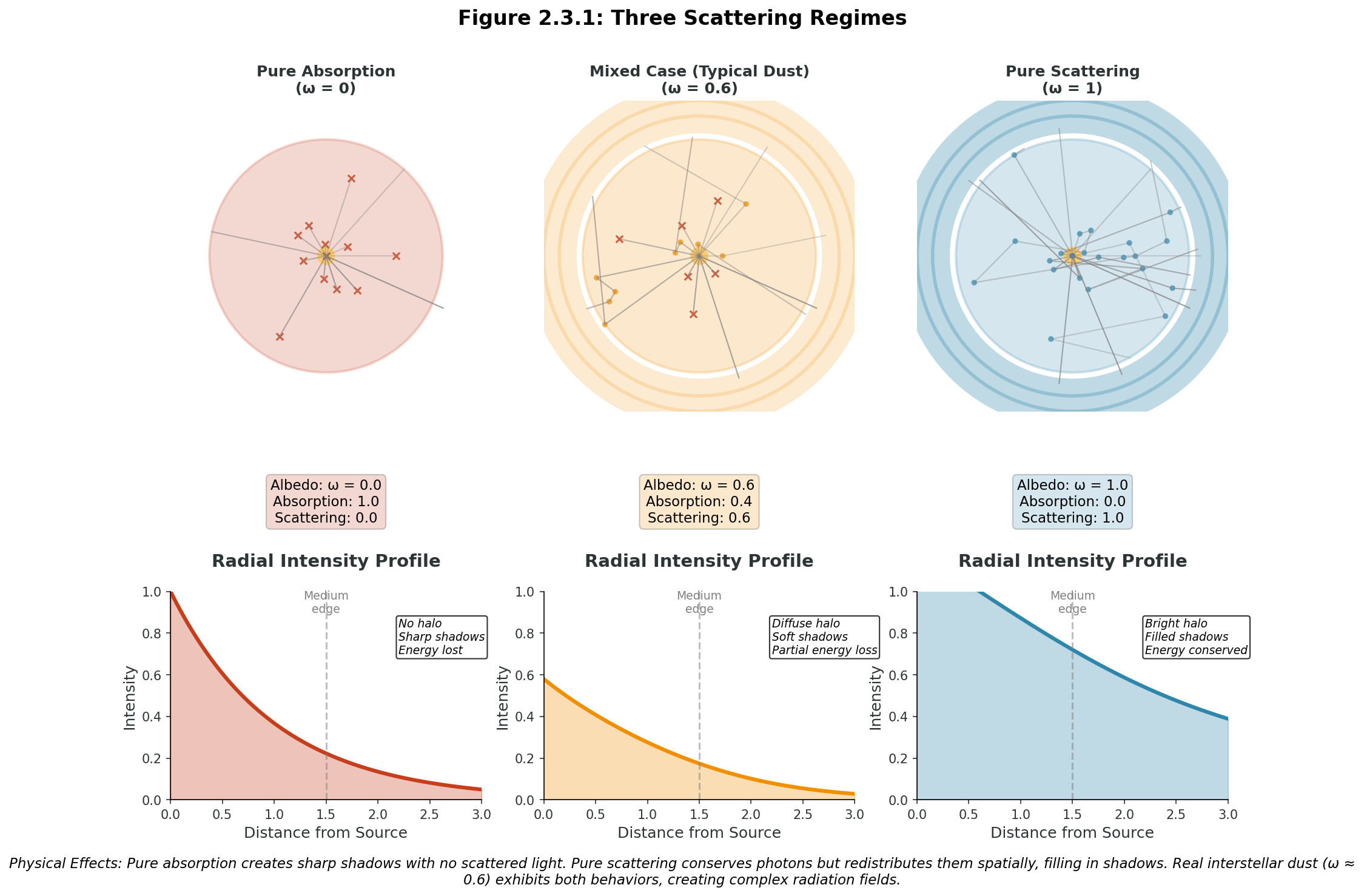
Define the single scattering albedo: \[\omega_\nu = \frac{\kappa_\nu^{\text{sca}}}{\kappa_\nu^{\text{ext}}}\]
This gives the probability that an interaction is scattering rather than absorption:
- \(\omega = 0\): Pure absorption — “black” (all photons destroyed, no scattering)
- \(\omega = 1\): Pure scattering — “white” (all photons redirected, no absorption)
- \(0 < \omega < 1\): Mixed (typical for dust, e.g., \(\omega = 0.6\) means 60% scatter, 40% absorb)
The concept of albedo appears throughout astrophysics. Here are typical values:
| Material/Context | Wavelength | Albedo (ω) | Physical Meaning |
|---|---|---|---|
| Interstellar Dust | |||
| ISM dust | UV (0.2 \(\mu\mathrm{m}\)) | ~0.7 | Strong scattering (why reflection nebulae appear blue) |
| ISM dust | Optical (0.55 \(\mu\mathrm{m}\)) | ~0.6 | 60% scatter, 40% absorb |
| ISM dust | Near-IR (2.2 \(\mu\mathrm{m}\)) | ~0.3 | Less scattering at longer λ |
| ISM dust | Far-IR (100 \(\mu\mathrm{m}\)) | ~0.01 | Almost pure absorption |
| Planetary Atmospheres | |||
| Earth clouds | Visible | ~0.8 | High reflectivity (why clouds appear white) |
| Venus clouds | Visible | ~0.76 | Sulfuric acid droplets scatter strongly |
| Mars dust | Visible | ~0.63 | Iron oxide gives reddish color |
| Surfaces (Bond albedo) | |||
| Fresh snow | Visible | ~0.9 | Highly reflective |
| Ocean water | Visible | ~0.06 | Strongly absorbing |
| Moon regolith | Visible | ~0.12 | Dark, absorbing surface |
| Earth (average) | Visible | ~0.31 | Combined clouds, ocean, land |
Key insight: In planetary science, “albedo” often refers to the Bond albedo — the fraction of total incident energy reflected by a planet. This is related to but different from the single scattering albedo \(\omega\) we use in radiative transfer. The connection: multiple scatterings with high \(\omega\) lead to high reflectivity (Bond albedo).
Physical interpretation: Materials with \(\omega\) close to 1 appear bright/white because they scatter light efficiently. Materials with \(\omega\) close to 0 appear dark/black because they absorb light. This is why fresh snow (\(\omega \approx 0.9\)) looks white while soot (\(\omega \approx 0.05\)) looks black!
The complete RTE becomes:
\[\frac{dI_\nu}{d\tau_\nu} = -I_\nu + (1-\omega_\nu)S_\nu^{\text{thermal}} + \omega_\nu \int_{4\pi} \frac{p(\hat{n}', \hat{n})}{4\pi} I_\nu(\hat{n}') \, d\Omega'\]
Isotropic Scattering: The Simplest Case
For isotropic scattering, \(p = 1\) (equal probability in all directions). The scattering source becomes:
\[j_\nu^{\text{sca}} = \frac{\omega_\nu}{4\pi} \int_{4\pi} I_\nu(\hat{n}') \, d\Omega' = \omega_\nu J_\nu\]
The RTE simplifies to:
\[\frac{dI_\nu}{d\tau_\nu} = -I_\nu + S_\nu^{\text{eff}}\]
with effective source function: \[S_\nu^{\text{eff}} = (1-\omega_\nu)S_\nu^{\text{thermal}} + \omega_\nu J_\nu\]
This is an integro-differential equation — \(I_\nu\) depends on \(J_\nu\), which depends on \(I_\nu\) in all directions!
Without scattering, each light ray evolves independently — radiation traveling north doesn’t affect radiation traveling south.
With scattering, rays become coupled. A photon traveling north can scatter and start traveling south. This means:
- Can’t solve one direction at a time
- Need iteration or Monte Carlo methods
- Computational cost increases dramatically
- But creates beautiful effects like halos around stars!
The coupling happens because \(J_\nu\) in the source function depends on the intensity in ALL directions. To find \(I_\nu\) in one direction, we need to know \(I_\nu\) everywhere!
 {#fig:scattering_regimes width=“100%” fig-align=“center”}
Consider a bright star embedded in a dusty nebula. Without scattering, the star would cast sharp shadows. But with scattering, something remarkable happens.
Mental experiment: Imagine you’re looking at a region that’s in the “shadow” of a dust clump.
Question: With \(\omega = 0.8\) (typical for dust), will this shadow region be completely dark?
No. Scattered light will partially fill in the shadow. Photons from the star can scatter around the dust clump and reach the “shadow” region. This is why shadows in dusty regions appear soft and diffuse, not sharp. The higher the albedo, the more scattered light fills in shadows.
This non-locality is what makes scattered light problems computationally expensive — you can’t just trace rays independently. Every point receives scattered light from every other point. This is why Monte Carlo methods are so valuable for these problems — they naturally handle this coupling.
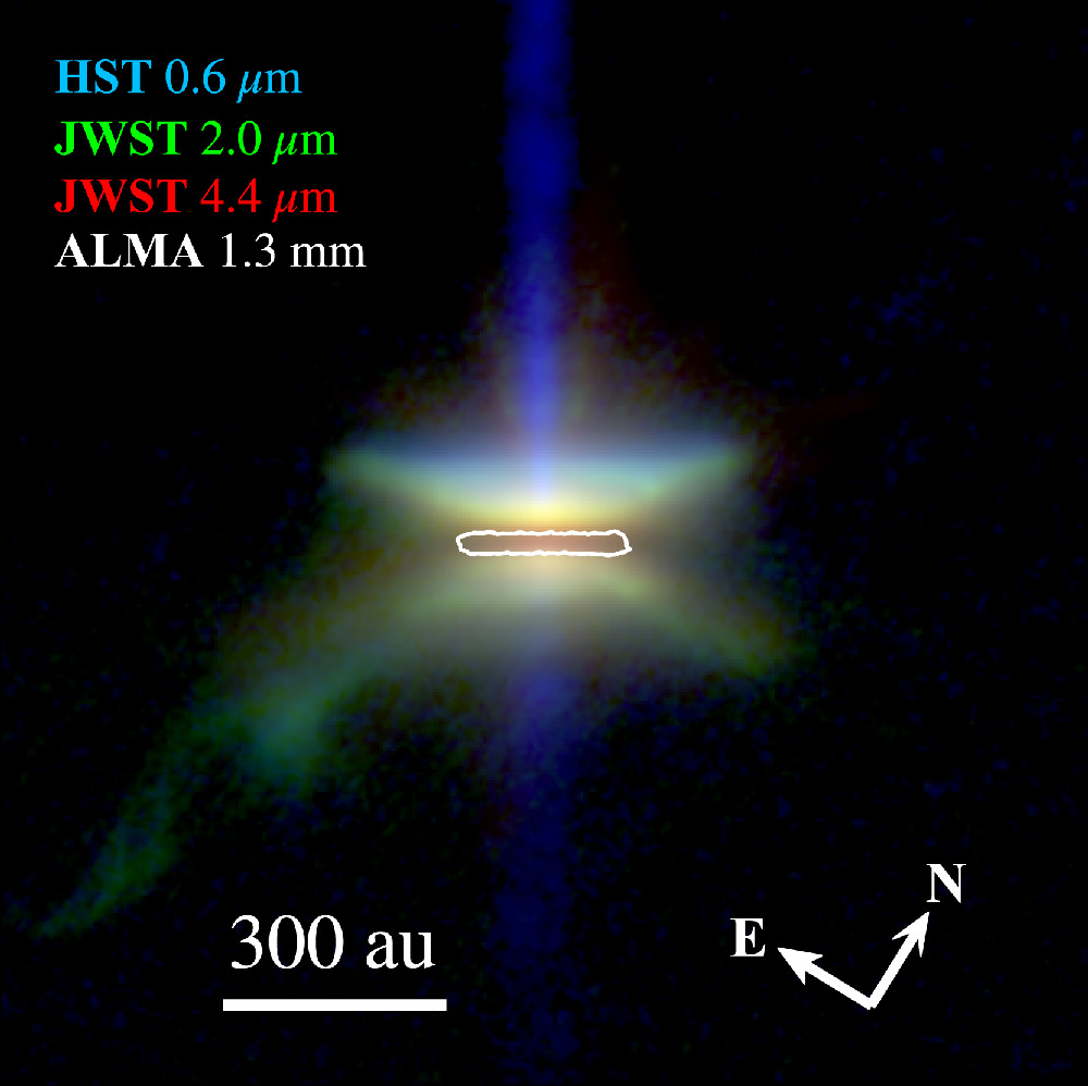 {#fig:hh30-scattered-light width=“100%”}
Quick Check 2.3
Test your understanding of scattering in radiative transfer:
Level 1 - Conceptual: a) What does albedo \(\omega = 0.6\) mean physically? b) Why does pure scattering (\(\omega = 1\)) conserve photons? c) How does scattering couple different directions?
Level 2 - Calculation: A medium has \(\omega = 0.5\), thermal source \(S^{\text{thermal}} = 100\), and mean intensity \(J = 80\). a) Calculate the effective source function b) Find the scattering contribution to emission c) What fraction of extinction is due to absorption?
Level 3 - Application: For dust with \(\omega_V = 0.6\) at visual wavelengths: a) If 1000 photons interact, how many scatter vs absorb? b) Derive the albedo at 2.2 \(\mu\mathrm{m}\) if \(\omega \propto \lambda^{0.3}\) c) Explain why infrared observations penetrate dust better
Click for solutions
Level 1 Answers: a) 60% of interactions are scattering, 40% absorption b) Photons change direction but aren’t destroyed - total number conserved c) Scattered photons from one direction become sources for other directions
Level 2 Solutions: a) Effective source function: \[S^{\text{eff}} = (1-\omega)S^{\text{thermal}} + \omega J = 0.5 \times 100 + 0.5 \times 80 = 90\]
Scattering contribution: \(\omega J = 0.5 \times 80 = 40\) units
Absorption fraction: \(1 - \omega = 0.5\) (50%)
Level 3 Solutions: a) Scattering: \(1000 \times 0.6 = 600\) photons Absorption: \(1000 \times 0.4 = 400\) photons
At 2.2 \(\mu\mathrm{m}\): \[\omega_{2.2} = \omega_V \times (2.2/0.55)^{0.3} = 0.6 \times 4^{0.3} \approx 0.6 \times 1.52 = 0.91\]
Higher albedo + lower opacity means:
- Less absorption (higher \(\omega\))
- Lower total extinction (dust more transparent)
- Combined effect: much better penetration!
Here’s a subtle but crucial point about pure scattering \((\omega = 1)\):
Question: If a medium only scatters light (no absorption), and you surround a light source completely with this medium, where does the energy go?
Think before reading on…
All the energy eventually escapes! Pure scattering conserves photon number and energy. Photons may take longer to escape (random walk), and they emerge in different directions than they started, but every photon that goes in must come out. This is why Earth’s clouds (which mostly scatter) don’t violate energy conservation — they redirect sunlight but don’t destroy it.
Follow-up: What would you observe if you looked at a bright star through a purely scattering medium?
You’d see:
- The star appears dimmer (flux redistributed to larger angles)
- A bright halo surrounds the star (scattered light)
- The integrated flux (star + halo) equals the original flux
- The star might appear slightly shifted or distorted
This is exactly what we see with bright stars near nebulosity!
Important: Common Pitfalls to Avoid
Before synthesizing everything, let’s address the most common conceptual and computational errors students make:
1. Confusing Optical Depth with Physical Depth.
- ❌ Wrong: “\(\tau = 5\) means the cloud is 5 parsecs thick”
- ✅ Right: “\(\tau = 5\) means five mean free paths, physical depth depends on density”
- Remember: \(\tau = \int \kappa \rho \, ds\) - same \(\tau\) can mean different physical distances!
2. Forgetting the \(\cos\theta\) Factor in Flux.
- ❌ Wrong: \(F = \int I \, d\Omega\)
- ✅ Right: \(F = \int I \cos\theta \, d\Omega\)
- The \(\cos\theta\) accounts for projected area - crucial for energy conservation!
3. Missing the \(4\pi\) in Mean Intensity.
- ❌ Wrong: \(J = \int I \, d\Omega\) (this would have units of flux!)
- ✅ Right: \(J = \frac{1}{4\pi} \int I \, d\Omega\)
- The \(1/4\pi\) makes \(J\) have the same units as \(I\) (intensity)
4. Assuming Source Function Always Equals Planck Function.
- ❌ Wrong: “\(S = B(T)\) always”
- ✅ Right: “\(S = B(T)\) only in LTE; generally \(S\) depends on radiation field”
- Non-LTE is common in stellar atmospheres and nebulae!
5. Treating Scattering Like Absorption.
- ❌ Wrong: “Scattering removes photons, so treat it like absorption”
- ✅ Right: “Scattering redirects photons - they couple different directions”
- This coupling is why scattering problems need special methods
6. Using Wrong Units or Mixing Unit Systems.
- ❌ Wrong: Mixing CGS and SI units without conversion
- ✅ Right: Stay in one system (we use CGS) and track units explicitly
- Always verify dimensions balance in your equations!
7. Assuming Intensity Decreases with Distance.
- ❌ Wrong: “Distant objects have lower intensity”
- ✅ Right: “Intensity is conserved along rays; flux decreases as 1/r²”
- This is why we can measure surface brightness of distant galaxies!
8. Ignoring Frequency Dependence.
- ❌ Wrong: “If \(\tau = 1\) in optical, it’s 1 everywhere.”
- ✅ Right: “\(\tau\) is strongly wavelength dependent.”
- This wavelength dependence is why multi-wavelength astronomy works!
Remember: These aren’t just mathematical nitpicks - each represents a fundamental physical principle. Getting these right is the difference between code that works and code that seems to work but gives wrong answers!
Frequent unit mistakes to avoid:
- Mixing wavelength and frequency units:
- ❌ Wrong: Using \(I_\nu\) with wavelength in denominator
- ✅ Right: \(I_\nu\) has Hz⁻¹, \(I_\lambda\) has cm⁻¹ (or Å⁻¹)
- Conversion: \(I_\lambda = I_\nu |d\nu/d\lambda| = I_\nu c/\lambda^2\)
- Forgetting steradians:
- Intensity has sr⁻¹, flux doesn’t
- Mean intensity \(J\) has same units as \(I\) (the 1/4π has implicit sr⁻¹)
- When integrating \(\int I d\Omega\), the sr from \(d\Omega\) cancels the sr⁻¹ from \(I\)
- Opacity confusion:
- Mass opacity \(\kappa\): cm²/g (cross-section per unit mass)
- Volume coefficient \(\kappa\rho\): cm⁻¹ (inverse mean free path)
- Cross-section \(\sigma\): cm² (effective area)
- Column density \(N\): cm⁻² (particles per unit area)
- CGS vs SI mixing:
- Stick to one system throughout!
- We use CGS: erg, cm, g, s, K
- SI would be: J, m, kg, s, K
- Never mix! (e.g., don’t use meters with ergs)
- Temperature units in exponentials:
- In \(e^{h\nu/kT}\), verify \(h\nu\) and \(kT\) have same units (both energy)
- Common error: forgetting to convert T to energy units
- Remember: \(kT\) in ergs = \(1.38 \times 10^{-16} \times T\)(K)
Part II Synthesis: The Complete Mathematical Framework
We’ve established the complete mathematical framework for radiative transfer. Let’s see how everything connects:
The Hierarchy of Quantities:
- Specific intensity \(I_\nu(\vec{r}, \hat{n}, t)\) is fundamental — contains all information
- Moments yield observables: flux (1st), energy density (0th/c), pressure (2nd/c)
- The RTE governs evolution: Including emission, absorption, and scattering
- Source functions encode physics: Thermal emission plus scattered radiation
The Master Equation: \[\frac{dI_\nu}{d\tau_\nu} = -I_\nu + S_\nu^{\text{eff}}\]
with:
- Optical depth: \(d\tau = \kappa_\nu \rho \, ds\)
- Effective source: \(S_\nu^{\text{eff}} = (1-\omega)S_\nu^{\text{thermal}} + \omega J_\nu\)
- Formal solution: \(I_\nu(\tau) = I_\nu(0)e^{-\tau} + \int_0^\tau S_\nu(\tau')e^{-(\tau-\tau')}d\tau'\)
This framework is universal — it describes:
- Stellar atmospheres (where developed) and interiors
- Interstellar medium (dust extinction and emission) - our focus for Project 3
- Planetary atmospheres (including Earth)
- Accretion disks
- Early universe (CMB)
- Medical imaging
- Neutron transport
The mathematics is always the same; only the physics determining \(\kappa\) and \(j\) changes!
Self-Assessment Checklist
Before proceeding to Part III (Monte Carlo Methods), verify you understand:
✅ Section 2.1: Statistical Description
▢ I can define specific intensity and explain its units
▢ I can calculate moments to get flux, energy density, pressure
▢ I understand why intensity is conserved along rays in vacuum
▢ I can perform angular integrations to derive flux from intensity
▢ I can distinguish between intensity (surface brightness) and flux (collected power)
✅ Section 2.2: Radiative Transfer Equation
▢ I can derive the RTE from conservation principles
▢ I understand optical depth as counting mean free paths
▢ I can solve simple cases (pure absorption, uniform source)
▢ I can apply the formal solution for practical problems
▢ I recognize the RTE as a Boltzmann equation for photons
▢ I can write pseudocode to solve the RTE numerically
✅ Section 2.3: Scattering
▢ I understand albedo as the scattering probability
▢ I can write the scattering source term for isotropic case
▢ I see how scattering couples the radiation field
▢ I recognize when iteration or Monte Carlo is needed
✅ Mathematical Connections
▢ I see how the RTE generalizes Beer’s law from Part I
▢ I understand the relationship between \(\tau\), \(A_\lambda\), and extinction
▢ I can connect mathematical formalism to Part I’s physical intuition
▢ I’m ready to implement these equations numerically in Part III and Project 3
Carry this forward: The RTE is conservation along a ray; \(\tau\) is the natural coordinate; scattering makes it non-local. When \(\tau \ll 1\), light passes freely. When \(\tau \gg 1\), only local sources matter.
In Part III, you’ll learn how to solve the RTE using Monte Carlo methods. The mathematical framework we’ve developed here — specific intensity \(I_\nu\), optical depth \(\tau\), source functions \(S_\nu\), scattering — will become the foundation for your computational implementation.
You’ll discover that the formal solution: \[I_\nu(\tau) = I_\nu(0)e^{-\tau} + \int_0^\tau S_\nu(\tau')e^{-(\tau-\tau')}d\tau'\]
naturally emerges from following individual photon/luminosity packets! Each Monte Carlo photon samples this equation statistically, and with enough photons, you recover the exact solution.
The key insight: Monte Carlo doesn’t approximate the RTE — it solves it exactly in the limit of infinite photons. The error decreases as \(1/\sqrt{N}\), guaranteed by the Central Limit Theorem you learned in Module 1!
The radiative transfer equation represents one of physics’ great unifications. Developed independently for different problems:
- Schuster (1905): Stellar atmospheres
- Schwarzschild (1906): Radiative equilibrium
- Milne (1921): Stellar interiors
- Chandrasekhar (1950): Complete theory
Each thought they were solving a specific problem, but they discovered universal mathematics. The same equation describes:
- Photons in stars
- Neutrons in reactors
- Light in Earth’s atmosphere
- X-rays in medical imaging
- Radiation in the early universe
This universality isn’t coincidence — it reflects deep mathematical structure. Any time you have particles (or waves) propagating through a medium that can absorb and emit them, you get the RTE. The physics changes (what determines \(\kappa\) and \(j\)), but the mathematics remains.
Your journey from physical intuition (Part I) through mathematical formalism (Part II) to computational implementation (Part III) mirrors the historical development of the field. But you’re completing in weeks what took humanity decades to understand!
Part II Resources
Main Takeaways
The Big Picture:
- Specific intensity \(I_\nu(\vec{r}, \hat{n}, t)\) is the fundamental quantity — it contains complete information about the radiation field
- All observables are moments: Flux (1st), energy density (0th/c), and pressure (2nd/c) emerge from integrating specific intensity
- The RTE is universal: One equation governs all radiation transport, from stellar atmospheres to medical imaging
- Optical depth is the natural variable: Using \(\tau\) instead of physical distance simplifies the mathematics
- Scattering couples everything: It transforms a local problem into a global one, requiring special solution methods
Key Equations You Must Know:
| Equation | Form | Physical Meaning |
|---|---|---|
| Specific Intensity | \(I_\nu = \frac{dE}{dA \, dt \, d\nu \, d\Omega}\) | Energy flow per area, time, frequency, solid angle |
| RTE (physical) | \(\frac{dI_\nu}{ds} = -\kappa_\nu \rho I_\nu + j_\nu\) | Change = -absorption + emission |
| RTE (optical depth) | \(\frac{dI_\nu}{d\tau_\nu} = -I_\nu + S_\nu\) | Simplified form using \(\tau\) |
| Optical depth | \(d\tau = \kappa \rho \, ds\) | Dimensionless measure of opacity |
| Source function | \(S_\nu = j_\nu/(\kappa_\nu \rho)\) | Equilibrium intensity |
| Beer’s law | \(I = I_0 e^{-\tau}\) | Pure absorption solution |
| Formal solution | \(I(\tau) = I_0 e^{-\tau} + \int_0^\tau S(\tau')e^{-(\tau-\tau')}d\tau'\) | General RTE solution |
| Flux from intensity | \(F = \int I \cos\theta \, d\Omega\) | Observable from fundamental quantity |
Critical Insights: - When \(I_\nu = S_\nu\), we have radiative equilibrium (\(dI/ds = 0\)) - Intensity is conserved along rays in vacuum, flux decreases as \(1/r^2\) - The mean free path is statistical: \(P(\text{survive to } s) = e^{-s/\ell}\) - Albedo \(\omega\) determines scattering vs absorption probability - Scattering creates an integro-differential equation requiring iteration or Monte Carlo
Glossary of Terms
A:
Albedo (ω): Single scattering albedo; probability that an interaction is scattering rather than absorption. Range: [0,1] where 0 = pure absorption (“black”), 1 = pure scattering (“white”)
Absorption coefficient: See opacity
C:
Column density (N): Number of particles per unit area along a sight line. Units: cm⁻². Relates to optical depth via \(\tau = N\sigma\)
Cross-section (σ): Effective area for particle interaction. Units: cm²
E:
Effective source function: \(S_{\text{eff}} = (1-\omega)S_{\text{thermal}} + \omega J\), combining thermal emission and scattering
Emission coefficient (j_ν): Energy emitted per unit volume, time, frequency, and solid angle. Units: erg cm⁻³ s⁻¹ Hz⁻¹ sr⁻¹
Energy density (u_ν): Radiation energy per unit volume and frequency. \(u_\nu = (4\pi/c) J_\nu\). Units: erg cm⁻³ Hz⁻¹
Extinction: Combined effect of absorption and scattering that removes photons from a beam
F:
Flux (F_ν): Energy flow per unit area, time, and frequency. First moment of intensity. Units: erg cm⁻² s⁻¹ Hz⁻¹
Formal solution: General solution to the RTE for arbitrary source function
I:
Intensity: See specific intensity
Integro-differential equation: Equation containing both derivatives and integrals; RTE with scattering is an example
J:
- J_ν (mean intensity): Angle-averaged specific intensity. \(J_\nu = \frac{1}{4\pi}\int I_\nu d\Omega\). Units: same as intensity
K:
- Kirchhoff’s law: In thermal equilibrium, emission and absorption coefficients are related: \(j_\nu = \kappa_\nu \rho B_\nu(T)\)
L:
- LTE (Local Thermodynamic Equilibrium): Condition where collisions dominate, maintaining Maxwellian distributions. Source function equals Planck function: \(S_\nu = B_\nu(T)\)
M:
Mean free path (ℓ): Average distance a photon travels before interaction. \(\ell = 1/(n\sigma) = 1/(\kappa\rho)\). Units: cm
Moments of intensity: Integrals of intensity weighted by powers of \(\cos\theta\). 0th moment \(\to\) energy density, 1st \(\to\) flux, 2nd \(\to\) pressure
O:
Opacity (\(κ_ν\)): Mass absorption/scattering coefficient. Cross-section per unit mass. Units: cm² g⁻¹
Optical depth (\(τ\)): Dimensionless measure of opacity. \(\tau = \int \kappa \rho \, ds\). When τ = 1, ~63% of photons have interacted
P:
Phase function \(p(n̂', n̂)\): Probability distribution for scattering from direction n̂’ to n̂. Normalized: \(\int p \, d\Omega/4\pi = 1\)
Planck function \(B_ν(T)\): Blackbody intensity. \(B_\nu = \frac{2h\nu^3}{c^2}\frac{1}{e^{h\nu/kT}-1}\)
Poisson process: Statistical process governing photon interactions; leads to exponential path length distribution
R:
Radiation pressure (P_ν): Momentum flux; second moment of intensity. \(P = u/3\) for isotropic radiation
Radiative equilibrium: Condition where \(I_\nu = S_\nu\), so \(dI/ds = 0\). Emission exactly balances absorption
Radiative Transfer Equation (RTE): Master equation governing radiation propagation: \(\frac{dI_\nu}{d\tau_\nu} = -I_\nu + S_\nu\)
S:
Scattering: Process redirecting photons without absorption. Elastic = no frequency change
Solid angle \((Ω)\):: 2D angle in 3D space. Units: steradian (sr). Full sphere = 4π sr
Source function \((S_ν)\): Ratio \(j_\nu/(\kappa_\nu\rho)\). Represents equilibrium intensity. In LTE, equals Planck function
Specific intensity \((I_ν)\): Fundamental quantity; energy flow per unit area, time, frequency, and solid angle. Units: erg cm⁻² s⁻¹ Hz⁻¹ sr⁻¹
T:
Transmission: Fraction of light passing through medium. \(T = e^{-\tau}\)
Transport equation: General name for equations like the RTE describing particle/wave propagation
V:
- Volume absorption coefficient: \(\kappa\rho\), absorption per unit length. Units: cm⁻¹
Quick Reference Formulas
Conversions:
- Intensity wavelength ↔︎ frequency: \(I_\lambda = I_\nu c/\lambda^2\)
- Optical depth ↔︎ extinction: \(\tau = 0.921 A_{\text{mag}}\)
- Column density ↔︎ optical depth: \(\tau = N\sigma\)
- Mean free path: \(\ell = 1/(\kappa\rho)\)
Key Relations:
- RTE (optical depth): \(\frac{dI_\nu}{d\tau_\nu} = -I_\nu + S_\nu\)
- Flux from intensity: \(F = \int I \cos\theta \, d\Omega\)
- Energy density: \(u = (4\pi/c) J\)
- Radiation pressure (isotropic): \(P = u/3\)
- Survival probability: \(P(s) = e^{-\tau}\)
- Scattering probability: \(P_{\text{sca}} = \omega\)
Typical Values (ISM):
- Standard \(R_V = 3.1\) (diffuse ISM), Dense clouds \(R_V = 4\)–\(5.5\)
- Dust albedo: \(\omega_V \approx 0.6\)
- Column to V-band optical depth: \(\tau_V \approx 1.8 \times 10^{-21} N_H\)
- Infrared advantage: \(A_K/A_V \approx 0.11\)