Spectra & Composition
Complete lesson
Spectrum as Data
By the end of this reading, you will be able to:
Atoms are nature’s barcode readers — each element absorbs and emits light at a unique set of wavelengths determined by its electron energy levels. By measuring where spectral lines appear and how they shift, we read a star’s composition and velocity from across the galaxy. And the same physics that decodes starlight explains why adding CO₂ to an atmosphere warms a planet.
Spectrum
The intensity of light as a function of wavelength, obtained by dispersing light through a prism or diffraction grating. A spectrum is quantitative data: its continuum slope, emission peaks, and absorption lines each encode physical conditions of the source.
Source Geometry
Part 1: Kirchhoff’s Laws — Why Stars Show Absorption Spectra
Three Types of Spectra
In Lecture 4 (Module 1), you saw a preview of spectral types. Now we formalize the physics. Light sources produce three distinct spectral signatures, depending on their structure:
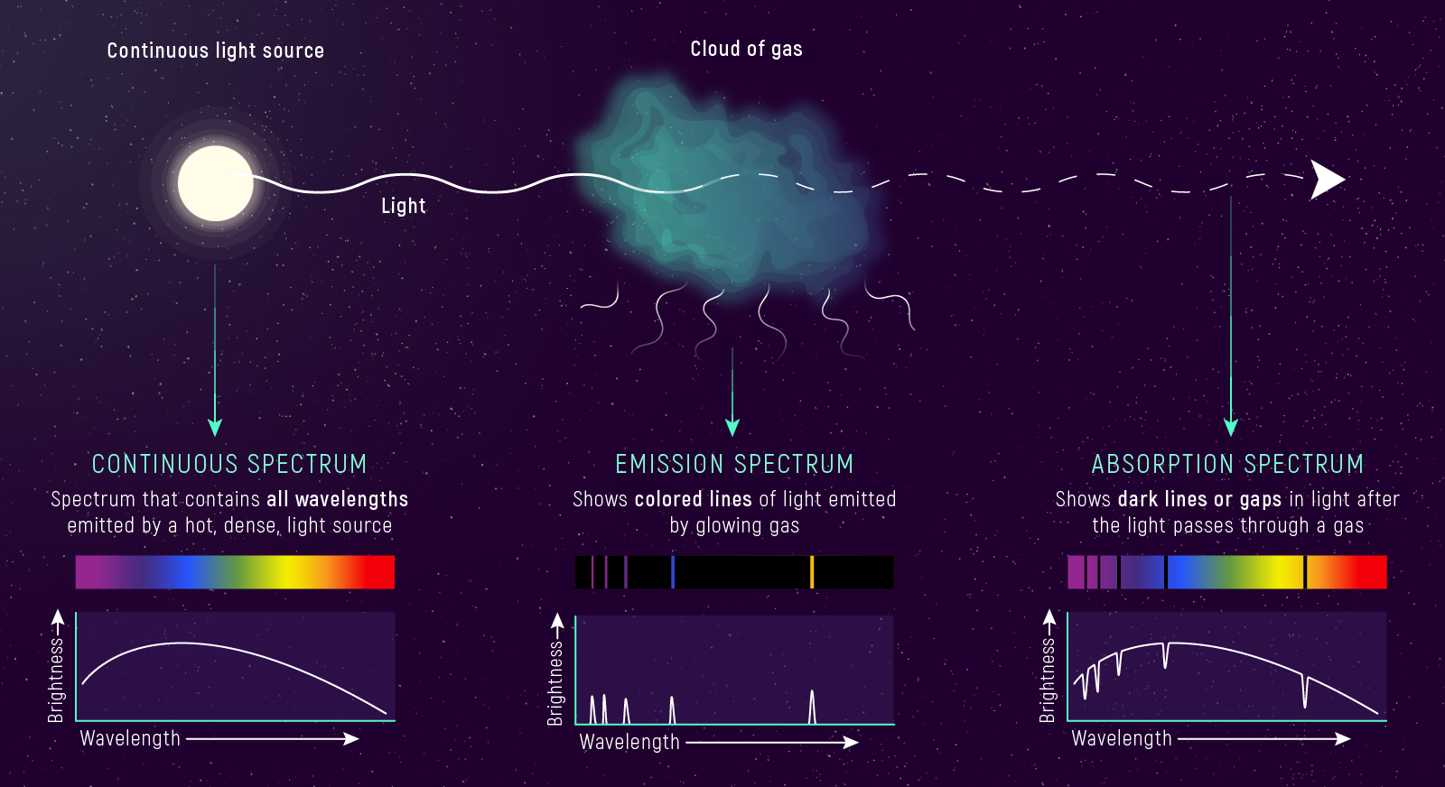
Continuous spectrum (blackbody continuum): a hot, dense source — a solid, liquid, or dense gas — emits light at all wavelengths, producing a smooth rainbow. The shape follows the Planck function you studied in Lecture 4 (Module 1). Examples: the Sun’s photosphere, an incandescent filament, the interior of a kiln.
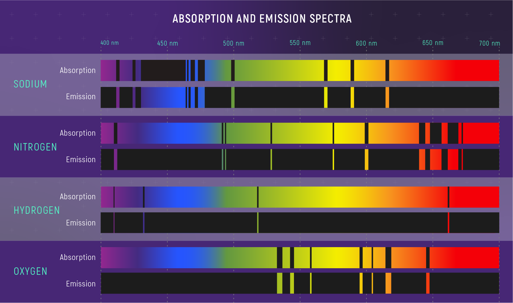
Emission spectrum (bright lines on a dark background): a hot, low-density gas emits photons only at specific wavelengths — those corresponding to transitions between its atoms’ energy levels. The background is dark; you see isolated bright lines. Examples: nebulae excited by nearby hot stars, neon signs, gas discharge tubes.
Absorption spectrum (dark lines in a continuous rainbow): a cooler gas in front of a hotter continuum source absorbs photons from the continuum at exactly the wavelengths it would emit if heated. You see the rainbow interrupted by dark lines — a photographic negative of the emission spectrum. Examples: stellar spectra, the solar spectrum (Fraunhofer lines).
Kirchhoff’s Laws of Spectroscopy
These three observations codify into
- A hot, dense object emits a continuous spectrum — all wavelengths, shaped by .
- A hot, low-density gas emits an emission-line spectrum — bright lines at wavelengths determined by its atomic composition.
- A cooler gas in front of a hot continuum source produces an absorption-line spectrum — the continuum minus specific wavelengths, at the same positions the gas would emit if heated.
Kirchhoff's laws
Three rules linking the appearance of a spectrum to the physical conditions of its source: (1) a hot dense object yields a continuous spectrum; (2) a hot low-density gas yields bright emission lines; (3) a cool gas in front of a hotter continuum yields dark absorption lines at the same wavelengths it would emit. Worked backward, a spectrum’s appearance reveals the source’s configuration.
Dark lines at specific wavelengths in a star's spectrum
A stellar spectrum is a continuous rainbow scored by dark absorption lines at precise, repeatable wavelengths.
Kirchhoff's third law
A cooler gas in front of a hotter continuum source absorbs at its characteristic wavelengths — the star’s atmosphere absorbs from the photosphere below.
A hot interior wrapped in a cooler atmosphere
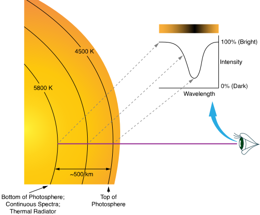
The star has a hot, dense continuum source (the photosphere) surrounded by a cooler absorbing layer (the atmosphere) — the two-layer structure that produces every stellar absorption line.
Why Stars Show Absorption Spectra: The Two-Layer Model
A star has a steep temperature gradient. Deep in the interior, temperatures reach millions of kelvin. The
Photosphere
The visible “surface” of a star — the depth at which it becomes opaque (optical depth ) and from which the continuous spectrum escapes. For the Sun it sits near 5,800 K; the slightly cooler atmosphere just above it carves the absorption lines.
The light we observe is emitted by the photosphere (Kirchhoff’s law 1, a continuous spectrum). As this light travels outward through the cooler atmosphere, atoms there absorb photons at their characteristic wavelengths (Kirchhoff’s law 3, dark absorption lines appear). The result: a continuous spectrum scored by dark absorption lines.
Quick check
- You observe a smooth rainbow with no dark lines. What type of source are you looking at?
- You observe bright colored lines on a dark background. What produces this?
- You observe a rainbow interrupted by dark lines at specific wavelengths. What’s happening physically?
- A hot, dense source (Kirchhoff’s law 1) — like an incandescent filament or a star’s photosphere viewed without its atmosphere.
- A hot, low-density gas (Kirchhoff’s law 2) — like a nebula or gas discharge tube.
- A cooler gas absorbing from a hotter continuum (Kirchhoff’s law 3) — like a stellar atmosphere in front of its photosphere. The dark lines tell you which atoms are in the cool gas.
Part 1 takeaway: Kirchhoff’s three laws connect the appearance of a spectrum to the physical conditions of the source. Stars produce absorption spectra because their cooler atmospheres absorb from the hotter photosphere — and those dark lines are the key to everything that follows.
Atomic Fingerprints
Part 2: Spectral Lines as Atomic Fingerprints
The Bohr Model and Discrete Energy Levels
Why do atoms absorb and emit at specific wavelengths rather than at all wavelengths? The answer comes from quantum mechanics: electrons in an atom occupy discrete energy levels — quantized rungs on an energy ladder. They cannot hover between rungs.
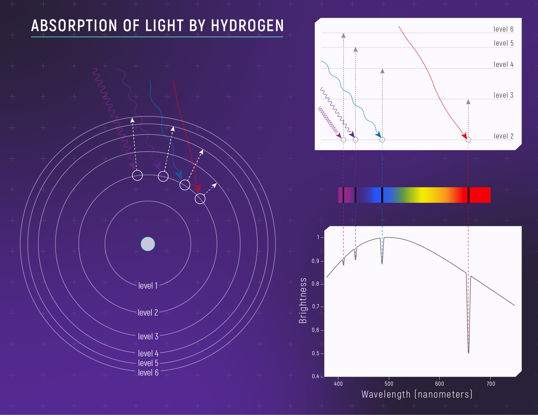
Now look at the reverse process — what happens when excited electrons fall back down through the energy levels:
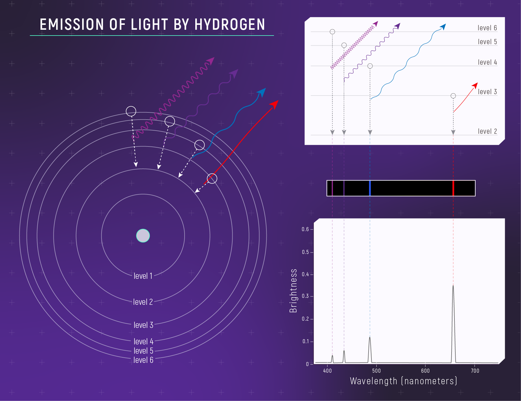
The same energy gaps produce the same wavelengths whether the photon is absorbed (electron jumps up) or emitted (electron falls down). This is why an
Absorption line
A dark feature in a spectrum where a cool gas absorbs photons from a hotter background source at a specific wavelength set by an atomic energy-level gap. It appears at the same wavelength the gas would emit if heated.
The
Here is the principal quantum number and 13.6 eV is the ionization energy of hydrogen — the energy needed to completely free the electron.
Bohr model
A quantum model of hydrogen in which the electron occupies discrete energy levels and absorbs or emits a photon only when it transitions between levels. Approximate for multi-electron atoms, but the core idea — discrete levels yield discrete lines — is exactly right.
Key observations from this equation:
- (ground state): — the most tightly bound level (most negative energy).
- (first excited state): — less tightly bound.
- As increases: levels crowd together and approach (the ionization threshold, where the electron is free).
- Negative sign: the electron is bound. You must add energy to free it.
When an electron transitions between levels, it absorbs or emits a photon whose energy equals the difference between the two levels:
The photon’s wavelength is set by the energy-wavelength relation:
Rearranging for wavelength gives .
This is the key insight: each transition produces a photon at a specific wavelength, set entirely by the energy gap between levels. Different elements have different energy-level structures (different nuclear charges, different electron configurations), so each element produces a unique set of spectral lines — a fingerprint as distinctive as DNA.
The Hydrogen Balmer Series: Visible Fingerprints
The most famous set of spectral lines in astronomy is the
| Transition | Name | Wavelength (nm) | Color |
|---|---|---|---|
| Hα | 656.3 | Deep red | |
| Hβ | 486.1 | Blue-green | |
| Hγ | 434.0 | Violet | |
| Hδ | 410.2 | Near-UV |
Balmer series
Hydrogen spectral lines from transitions to or from the level. The visible members are Hα (656 nm), Hβ (486 nm), Hγ (434 nm), and Hδ (410 nm) — the most prominent features in many stellar spectra.
These four lines are the most prominent features in the visible spectra of many stars. They fall in the visible range because the energy differences (about 1.9–3.0 eV) match the energy of visible photons.
Problem
Use the Bohr model to predict the wavelength of the transition in hydrogen. Compare to the observed Hα wavelength of 656.3 nm.
StepFind the energy levels
StepCompute the energy difference
StepConvert to CGS ($1\ \text{eV} = 1.602 \times 10^{-12}\ \text{erg}$)
StepApply $\lambda = hc/\Delta E$ and convert to nm
Dimensional check
✓.
Result
The Bohr model predicts Hα at 656 nm — within 0.3 nm of the precise laboratory value (656.28 nm). The small difference comes from rounding the ionization energy to 13.6 eV (the exact Rydberg value is 13.5984 eV). This agreement was one of the Bohr model’s great early triumphs, and the 1.89 eV gap lands squarely in the deep red.
Quick check
- An absorption line appears at 486.1 nm in a star’s spectrum. Which element and transition does it correspond to?
- If a hydrogen atom’s electron jumps from to , does the atom absorb or emit a photon? Is it visible?
- Why can’t hydrogen atoms absorb photons at any arbitrary wavelength?
- Hydrogen, Hβ (). The wavelength 486.1 nm is the second Balmer line.
- Absorbs — the electron moves up. The gap gives — deep ultraviolet, not visible (the Lyman series).
- Because energy levels are quantized — the electron can only occupy specific energies. A photon must have exactly the right energy (matching a level gap) to be absorbed; a “wrong” wavelength passes through unabsorbed.
Part 2 takeaway: atoms absorb and emit at specific wavelengths because electrons occupy discrete energy levels. Each element’s unique level structure creates a unique spectral fingerprint. By matching observed absorption lines to laboratory wavelengths, we identify which elements are present in a star’s atmosphere — without ever visiting the star.
Line Strengths
Part 3: The OBAFGKM Sequence — Temperature, Not Composition
A Temperature Sequence in Disguise
In the early 1900s, astronomers at Harvard Observatory — led by Annie Jump Cannon and Williamina Fleming — classified hundreds of thousands of stellar spectra by eye, sorting them by the appearance and strength of their spectral lines. After much rearranging, the sequence settled into O, B, A, F, G, K, M — from strongest helium lines to strongest molecular bands. The classic mnemonic: “Oh Be A Fine Guy/Girl, Kiss Me.”
The breakthrough came when Cecilia Payne-Gaposchkin showed in her 1925 PhD thesis — arguably the most important doctoral dissertation in the history of astronomy — that stars are overwhelmingly hydrogen and helium, and that the spectral sequence is fundamentally a temperature sequence, not a composition sequence. This was so radical that her advisor, Henry Norris Russell, initially urged caution (he later acknowledged she was right). Stellar composition is remarkably uniform (about 74% hydrogen, 25% helium, 1–2% heavier elements by mass). What changes along the sequence is not what atoms are present but which quantum states those atoms occupy — and that depends on temperature.
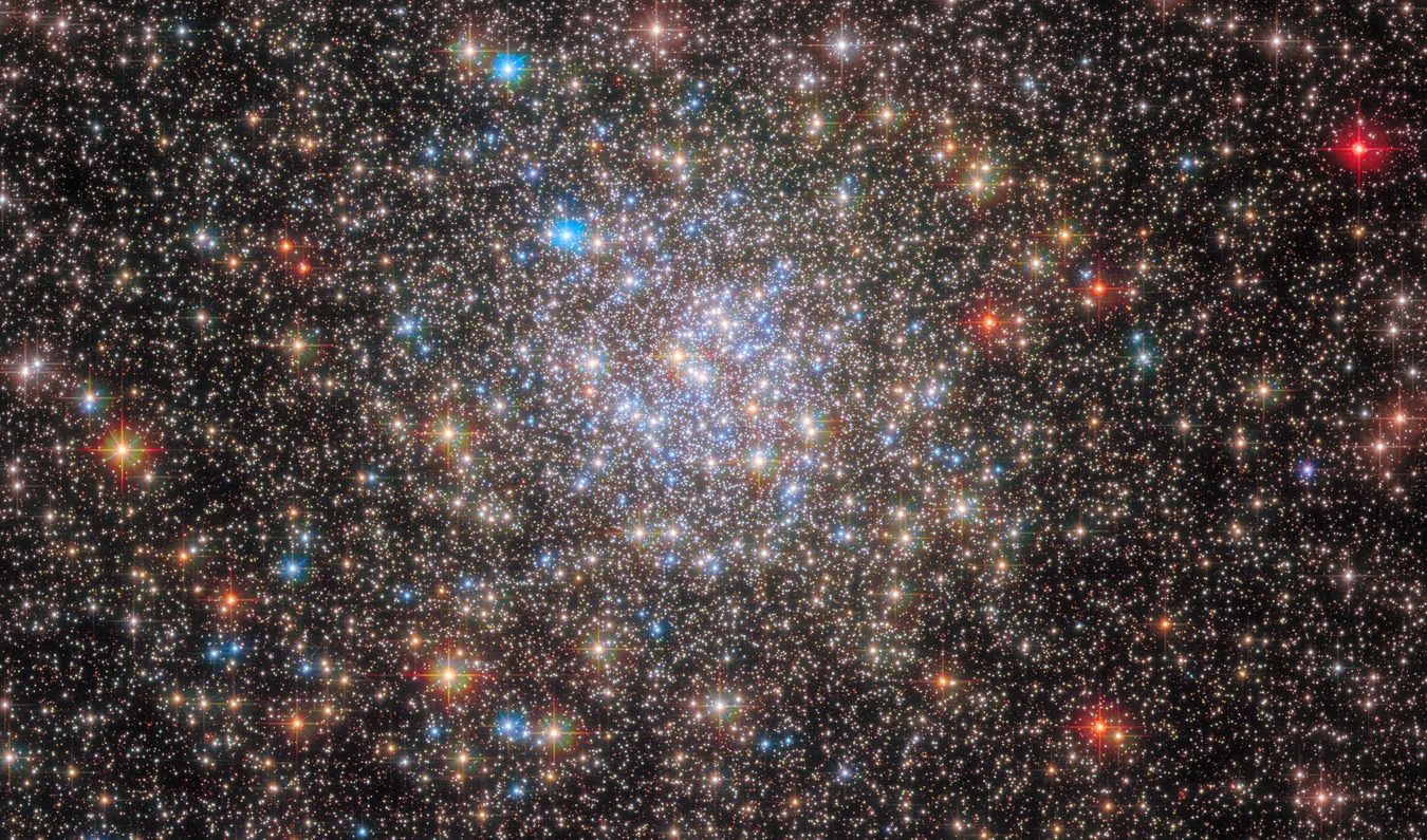
Before you read the sequence as letters in a table, look at the sky the way an observer does first: stars already announce that they are not thermally identical. A real star field shows blue-white, yellow, and orange-red stars sharing the same patch of sky. Spectroscopy explains why those colors differ, but the diversity is visible before any prism enters the story.
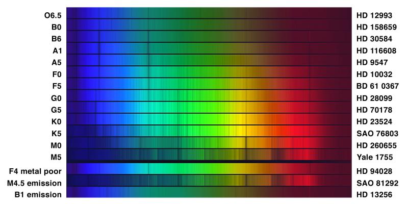
| Spectral Type | Color | Temperature Range | MS Prevalence | Dominant Features | Example |
|---|---|---|---|---|---|
| O | Blue-violet | 0.00003% | He II, weak H | O4I (ζ Puppis), O9.5V (10 Lac) | |
| B | Blue-white | 10,000–30,000 K | 0.13% | He I, strong H | B8Ia (Rigel), B1III (Spica) |
| A | White | 7,500–10,000 K | 0.6% | Strongest H Balmer lines | A1V (Sirius), A0V (Vega) |
| F | Yellow-white | 6,000–7,500 K | 3% | Moderate H, weak metals | F5IV (Procyon A) |
| G | Yellow | 5,200–6,000 K | 7.6% | Weak H, strong metal lines | G2V (Sun) |
| K | Orange | 3,700–5,200 K | 12.1% | Very weak H, strong metals, molecular bands appear | K1.5III (Arcturus) |
| M | Red-orange | 76.5% | Molecular bands (TiO), very weak H | M2Ia (Betelgeuse), M5V (Proxima Cen) |
Several examples are giants or supergiants rather than main-sequence dwarfs — those are the ones bright enough to have names. The prevalence column refers to main-sequence stars only.
Look at the prevalence column: M dwarfs make up over three-quarters of all main-sequence stars, yet they’re too faint to see with the naked eye. The bright stars that fill constellations — Rigel (B supergiant), Sirius (A dwarf), Arcturus (K giant) — are the rare luminous ones. The galaxy is dominated by cool, dim, long-lived M dwarfs.
Why Temperature Controls Line Strength
This is a critical conceptual point that trips up beginners: spectral type does NOT directly reflect composition. All main-sequence stars have roughly the same composition. What changes is which atomic transitions are active — and that depends on temperature through the
For an atom to absorb a photon at a given wavelength, an electron must already be in the right starting energy level. The fraction of atoms in any given level depends on temperature through the Boltzmann distribution:
where is the excitation energy — the energy above the ground state needed to reach level (always positive) — and is Boltzmann’s constant. For hydrogen, (the energy to excite from to ). Note is not the Bohr energy used earlier — it’s the gap , which is always positive.
Boltzmann distribution
The rule that the fraction of atoms in an excited level scales as , where is the excitation energy above the ground state. Its exponential sensitivity to temperature is why spectral type is a temperature sequence: temperature, not abundance, sets which levels are populated and therefore which lines appear.
The exponential is ruthless: even modest temperature changes dramatically shift which levels are populated. Higher excitation energy demands higher temperature for significant population. As a rough guide, every factor-of-two increase in temperature can boost high-energy level populations by orders of magnitude.
(More precisely, the full Boltzmann expression includes degeneracy factors and a partition function in the denominator, but the key physics — exponential sensitivity to — is captured above.)
Predict First
Commit to an answer before reading on.
The star-by-star walkthrough below confirms your reasoning.
How this creates the spectral sequence:
O stars (30,000+ K): so hot that collisions ionize most hydrogen — electrons are stripped free. No neutral hydrogen means weak Balmer lines. Instead we see lines of ionized helium (He II), which requires extreme temperatures. (The governing physics is the Saha equation, which we won’t derive — but the idea is simple: hot enough collisions knock electrons free entirely.)
A stars (7,500–10,000 K): the Goldilocks temperature for hydrogen Balmer absorption. Balmer strength reflects a competition between excitation and ionization: the Boltzmann factor sets what fraction of neutral atoms are in , while the Saha equation sets what fraction are neutral at all. At A-star temperatures, enough hydrogen stays neutral and enough of it is excited to that Balmer absorption is maximally efficient. H lines are strongest here.
G stars (5,800 K, like the Sun): Balmer lines are weaker — fewer atoms sit in . Metal absorption lines become prominent: ionized calcium (Ca II H & K at 393.4 and 396.8 nm), neutral iron, sodium (the D lines at 589.0 and 589.6 nm). The spectrum looks like a forest of metallic lines.
M stars (below 3,700 K): so cool that atoms stay neutral and even molecules form. Titanium oxide (TiO) produces broad absorption bands dominating the red and infrared. Balmer lines are very weak because almost no atoms are in .
Quick check
Your lab partner claims: “M stars have weak hydrogen lines because they have less hydrogen than A stars.” Construct a counterargument using the Boltzmann distribution. What fraction of hydrogen atoms are in at 3,000 K vs. 10,000 K?
At 3,000 K, , so — essentially zero atoms in . At 10,000 K, , so — tiny but significant. That’s a factor of difference in the Boltzmann factor with zero change in hydrogen abundance.
Metallicity: A Secondary Effect
Metallicity
The mass fraction of elements heavier than helium in a star or gas cloud (). It modulates the strength of metal absorption lines but, at fixed temperature, does not change a star’s spectral type — a second-order effect.
Quick check
- Which spectral type has the strongest hydrogen Balmer lines?
- Why are H lines weak in O stars — lack of hydrogen, or something else?
- Two stars have the same spectral type (G5). Must they have the same luminosity?
- A star’s spectrum shows strong TiO molecular bands. Is it hot or cool?
- A — the temperature (–) maximally populates the level.
- Something else — O stars have plenty of hydrogen, but it’s mostly ionized at 30,000+ K. No neutral hydrogen means no Balmer absorption.
- No — same type means similar temperature, but they could be a dwarf (V) or a giant (III) with luminosities differing by orders of magnitude. That’s why luminosity class exists.
- Cool — molecular bands form only at low temperatures (), characteristic of M-type stars.
Part 3 takeaway: OBAFGKM is a temperature sequence. Composition is nearly uniform across stars — what changes is which energy levels are populated, exponentially sensitive to temperature. Spectral type tells you temperature; metallicity and luminosity class add refinement.
Select all that apply
Give two physically distinct reasons a star could show very weak H Balmer lines, other than having less hydrogen.
Two reasons besides “less hydrogen”: (1) the star is too hot — hydrogen is ionized, so no neutral atoms exist for Balmer absorption (O stars); (2) the star is too cool — almost no hydrogen atoms are excited to (M stars). Both are temperature effects, not composition effects.
Line Shifts
Part 4: The Doppler Shift — Reading Stellar Motion from Light
The Doppler Effect for Light
You’ve experienced the Doppler effect with sound: an ambulance siren rises in pitch as it approaches and drops as it recedes. Light does the same. When a source moves toward or away from an observer, the observed wavelength shifts.
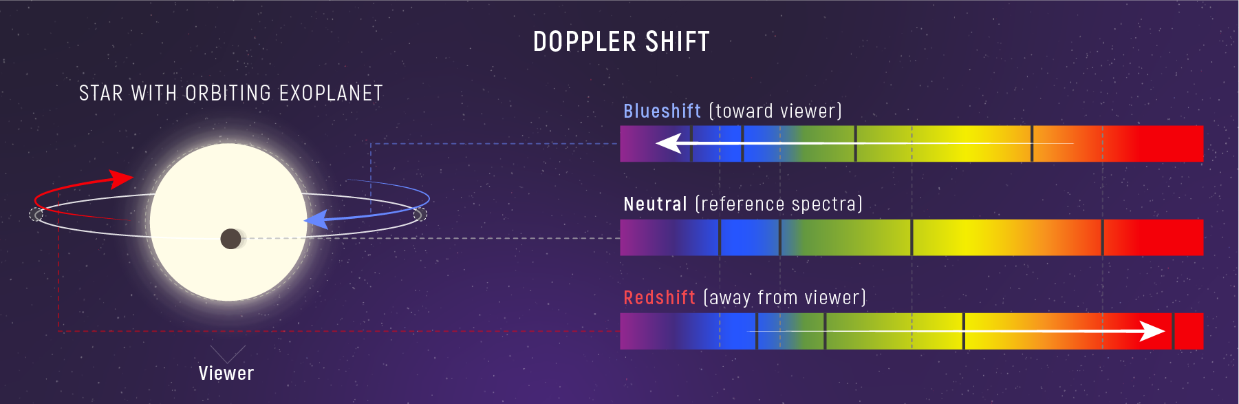
If a source has radial velocity (positive = receding, negative = approaching), the observed wavelength relates to the laboratory rest wavelength by the
Here , valid for (the non-relativistic limit), which covers virtually all stellar velocities in our galaxy.
Doppler shift
The change in observed wavelength caused by a source’s motion along the line of sight: . Receding sources shift to longer wavelengths (redshift); approaching sources shift to shorter wavelengths (blueshift).
Interpretation — shifts tell you direction:
Redshift Blueshift
Redshift
A shift of spectral lines to longer wavelengths (), indicating the source is receding from the observer.
Blueshift
A shift of spectral lines to shorter wavelengths (), indicating the source is approaching the observer.
Typical stellar radial velocities are 10–100 km/s; the speed of light is 300,000 km/s. The ratio to — tiny shifts, but measurable with precision spectrographs. For relativistic speeds (galaxies, jets, cosmology), a full relativistic formula is needed, and for the expanding universe the interpretation becomes cosmological redshift — a stretch of space itself, not simple motion. One crucial diagnostic: a real Doppler shift moves all lines by the same fractional amount . If only one line is shifted, it’s not motion — it’s a misidentification.
Problem
A nearby star’s Hα absorption line is observed at . The rest wavelength is . Is the star approaching or receding, and at what speed?
StepDetermine direction
Since exceeds , the line is redshifted — the star is receding.
StepWavelength shift, then solve for $v_r$
StepPlug in numbers
Dimensional check
✓.
Result
The star recedes at about 91 km/s — typical for the galactic disk. A shift of only 0.2 nm out of 656.3 nm (0.03%) translates to nearly 100 km/s because light is so fast. Modern spectrographs detect shifts 1,000 times smaller, reaching velocities of — precise enough to feel the tug of an orbiting exoplanet.
Lines shifted from their laboratory wavelengths
Absorption lines in a stellar spectrum appear at slightly different wavelengths than laboratory measurements — and all lines shift by the same fractional amount.
The non-relativistic Doppler effect
Motion along the line of sight shifts wavelengths by , valid for .
The star's radial velocity
The measured shift gives — the component of motion directly toward or away from us. Blueshift means approach; redshift means recession.
What Doppler Shifts Cannot Tell Us
The Doppler effect measures only the
Radial velocity
The component of a star’s velocity along the observer’s line of sight, measured from the Doppler shift of its spectral lines. The perpendicular (transverse) motion produces no shift and must be measured astrometrically.
Also, if a star is rotating, one limb moves toward you and the other away. This doesn’t shift the line center — it broadens the line symmetrically. Line broadening tells us about rotation speed and turbulence, but it’s a separate measurement from the Doppler shift of the line center.
Problem
- A star’s Hβ line (rest 486.1 nm) is observed at 485.9 nm. Is the star approaching or receding?
- Calculate the radial velocity for the star in question 1.
- Can we determine a star’s rotation rate from a single Doppler shift? Why or why not?
- Approaching — , so the light is blueshifted.
- . The negative sign confirms approach; the speed is .
- No — rotation broadens lines symmetrically (one limb approaches, the other recedes). A single shift of the line center gives only the bulk radial motion; rotation comes from the line width.
Doppler Applied: Detecting an Unseen Companion
So far we’ve measured a single Doppler shift — one velocity at one moment. But suppose you observe the same star night after night and its radial velocity changes periodically: the Hα line oscillates back and forth around the rest wavelength on a regular cycle. What could cause that? If the star has an orbiting companion — another star or a planet — gravitational tugs pull it toward us during part of the orbit and away during the rest. The result is a periodic Doppler oscillation whose amplitude tells you how fast the star moves and whose period tells you the orbital period.
Problem
You monitor a star over several weeks. Its Hα line () oscillates between 656.25 nm and 656.35 nm with a period of 4.0 days. (a) What is the velocity amplitude of the wobble? (b) What does the periodicity tell you?
Step(a) Convert the wavelength swing to a velocity
The line oscillates by around rest, so
Dimensional check
✓.
Result
(a) The radial velocity oscillates between (receding) and (approaching) — an amplitude of 23 km/s. (b) A periodic oscillation means the star orbits an unseen companion; the 4.0-day period is the orbital period. This is how the first exoplanet around a Sun-like star, 51 Pegasi b, was found in 1995 — its host wobbled with a 56 m/s amplitude over 4.23 days, 400 times smaller than this example. Repeated Doppler measurements reveal orbits, and orbits — through Kepler’s laws — give masses. This is the bridge to Lecture 4.
Part 4 takeaway: the Doppler shift formula converts tiny wavelength shifts into stellar velocities. Blueshifts mean approach; redshifts mean recession. This tool unlocks binary star masses in Lecture 4 and, on cosmological scales, reveals the expansion of the universe.
Spectrum Inference
Part 5: Putting It Together — Reading a Real Stellar Spectrum
You now have a complete spectroscopic toolkit. A single stellar spectrum gives you three independent pieces of information:
| Observable | What we measure | What we infer |
|---|---|---|
| Which lines appear (wavelength positions) | Line wavelengths matched to lab data | Composition — which elements are present |
| How strong lines are (depth and pattern) | Relative strengths of different species | Temperature (spectral type) — which states are populated |
| Where lines are shifted (offset from lab) | Doppler shift | Radial velocity — motion toward/away |
Additional information comes from line widths (pressure, rotation, turbulence) and line splitting (Zeeman effect from magnetic fields), but the three inferences above are the workhorses.
Spectra are powerful but limited. Spectroscopy alone does not directly give luminosity (need distance + photometry), mass (need binary orbits or asteroseismology), radius (need Stefan-Boltzmann with and ), distance (need parallax or standard candles), or transverse velocity (need astrometric tracking).
Now let’s use all three clues simultaneously on a real problem.
Problem
You observe a star and measure: a blackbody continuum fit of ; strong Hα, Hβ, Hγ absorption; weak metal lines; and the Hα center at 656.1 nm (rest 656.3 nm). What can you infer?
Step(a) Spectral type
The temperature () and strong Balmer lines point to spectral type A — the Goldilocks temperature for hydrogen absorption. Weak metal lines are consistent.
Step(b) Radial velocity
Dimensional check
✓; the sign carries the direction.
Result
A hot A-type star, made mostly of hydrogen (like all stars), approaching at . To complete the picture you’d still need distance (parallax → luminosity), luminosity + temperature (→ radius via Stefan-Boltzmann), and time-series Doppler (→ binary companion → mass). Spectroscopy confirms and sharpens what color alone suggested.
Planetary Spectroscopy
Part 6: Spectroscopy Meets Climate — Why CO₂ Warms Planets
Everything you’ve learned about spectral absorption applies not only to stars but to planetary atmospheres. The same quantum physics that creates stellar absorption lines also creates the greenhouse effect — one of the most consequential applications of spectroscopy in all of science.
Planetary Energy Balance: Stefan-Boltzmann Applied to Planets
In Lecture 2, you learned the Stefan-Boltzmann law . It applies to any blackbody — and, to first approximation, a planet is one. A planet doesn’t generate its own luminosity; it absorbs sunlight and re-radiates that energy as thermal (blackbody) radiation in the infrared. The Sun and Earth are both approximate blackbodies, but at very different temperatures: the Sun’s Planck curve peaks in visible light (~0.5 μm), Earth’s in the thermal infrared (~10 μm). These two blackbody spectra barely overlap — and that spectral separation is what makes the greenhouse effect possible.
At energy balance, the planet radiates exactly as much as it absorbs. The power absorbed is built from three factors: the stellar flux at the planet’s distance ; the intercepted cross-section (the area of the shadow the planet casts, not its full surface); and the albedo correction , where the
This is — the blackbody temperature the planet would have with no atmosphere. The planet’s radius cancels entirely; only , , and remain.
Albedo
The fraction of incident light a surface or planet reflects rather than absorbs. is perfect absorption; is a perfect mirror. The Moon has , Earth , Venus . Only the absorbed fraction heats the planet.
Equilibrium temperature
The temperature at which a planet radiates exactly as much energy as it absorbs from its star, assuming no atmosphere: . The greenhouse effect raises the real surface temperature above this baseline.
The Greenhouse Effect: Absorption Lines in the Atmosphere
Earth’s surface radiates as an approximate blackbody at 288 K. Wien’s law gives the peak wavelength:
This is deep in the thermal infrared — far from the visible band where sunlight arrives. The figure below makes the separation vivid: the Sun’s incoming Planck curve (peaking near 0.5 μm) and Earth’s outgoing curve (peaking near 10 μm) barely overlap.
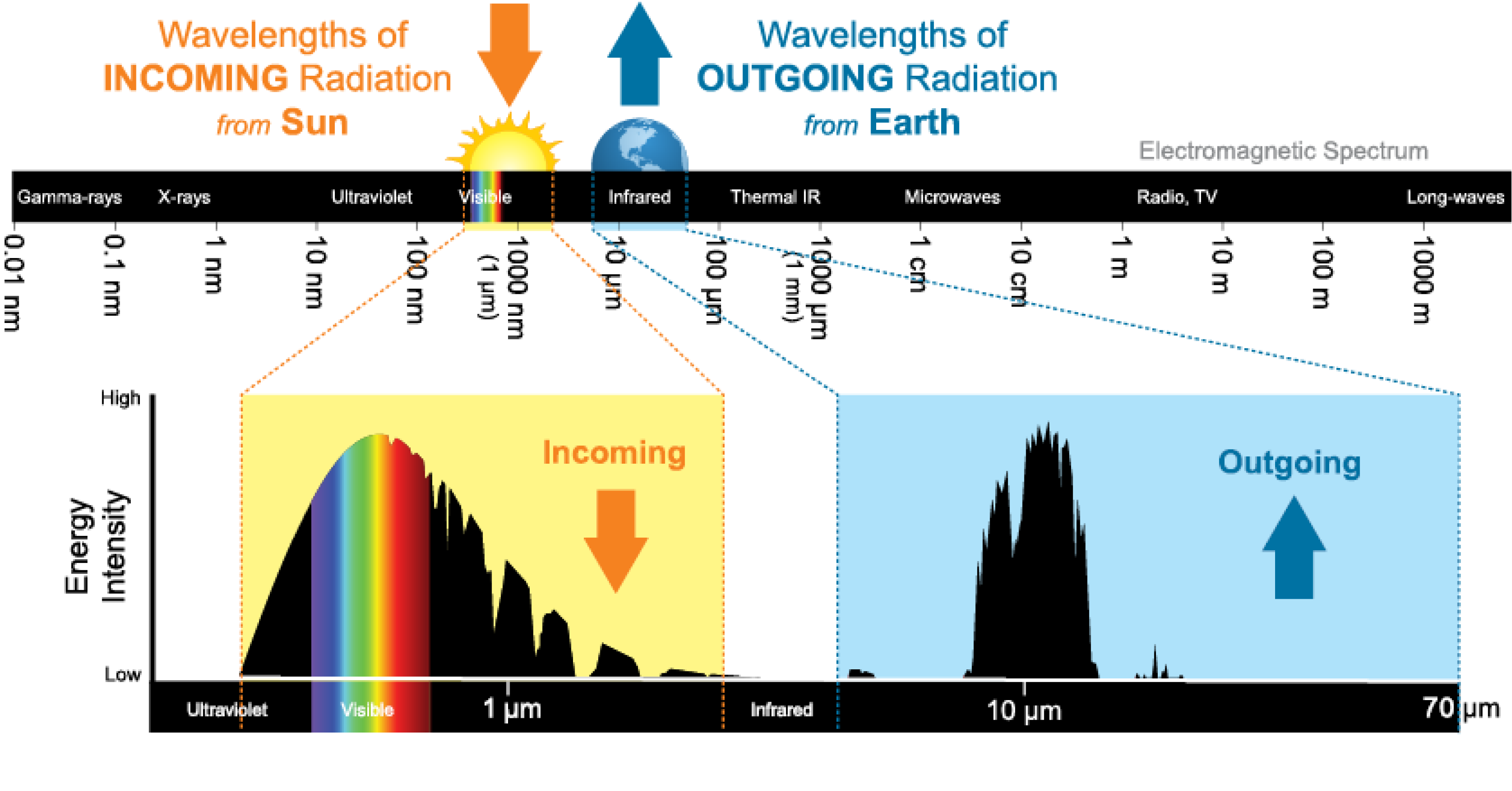
For Earth to maintain balance, this outgoing infrared must escape to space. But greenhouse gases — CO₂, H₂O, CH₄, N₂O — have molecular absorption bands in the infrared, precisely where Earth’s blackbody curve radiates. These molecules absorb outgoing infrared photons and re-emit them in random directions — some back downward. The surface receives extra energy and warms until it radiates enough to compensate.
Greenhouse effect
Warming of a planet’s surface caused by atmospheric gases absorbing outgoing infrared radiation and re-emitting part of it back downward. It is Kirchhoff’s third law applied to a planet: a cool atmosphere absorbing from the warm surface continuum.
A Tale of Three Planets
Venus, Earth, and Mars orbit the same star and formed from the same disk — yet their surface temperatures are wildly different. Spectroscopy tells us why:
| Planet | Distance (AU) | Albedo | (K) | Actual (K) | Greenhouse warming (K) | Dominant greenhouse gas |
|---|---|---|---|---|---|---|
| Venus | 0.72 | 0.77 | 227 | 735 | +508 | CO₂ (96.5% of atmosphere) |
| Earth | 1.00 | 0.30 | 255 | 288 | +33 | H₂O + CO₂ (0.04%) |
| Mars | 1.52 | 0.25 | 210 | 210 | ~0 | CO₂ (95%, but very thin) |
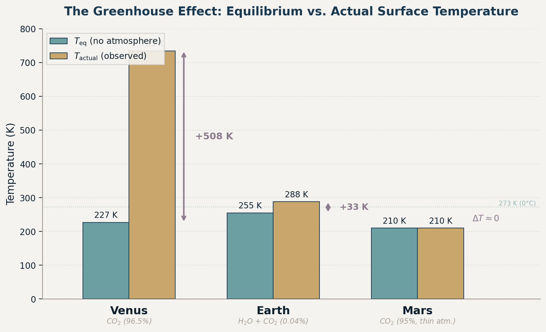
Venus is closer to the Sun than Earth, yet its equilibrium temperature is lower (227 K vs. 255 K). How? Albedo. Venus’s thick sulfuric-acid clouds reflect 77% of incoming sunlight before it can be absorbed. The factor means only the absorbed fraction matters: Venus absorbs just 23%, Earth 70%. The higher albedo more than compensates for the shorter distance — making the +508 K greenhouse warming even more staggering. Venus’s massive CO₂ atmosphere creates a runaway greenhouse: surface temperatures hot enough to melt lead (735 K = 462°C). Mars has a CO₂-dominated atmosphere too, but it’s so thin (0.6% of Earth’s surface pressure) that its greenhouse effect is negligible. Earth sits in between — a modest greenhouse that makes the planet habitable.
Problem
Calculate Earth’s equilibrium temperature assuming no atmosphere. Use , , and .
StepNumerator
StepDenominator
StepSolve for $T_{\text{eq}}$
Dimensional check
✓.
Result
. Without an atmosphere, Earth would be a frozen world. The observed average of 288 K (+15°C) means the greenhouse effect warms Earth by 33 K — the difference between a habitable planet and an ice ball, supplied by the infrared absorption bands of water vapor, CO₂, and other trace gases.
Predict First
Think about Kirchhoff's third law applied to a planet.
The 15-micron band below is the key.
Why CO₂ Matters: The 15-Micron Band
Carbon dioxide has a particularly strong absorption band centered at (15,000 nm). This sits right near the peak of Earth’s outgoing thermal radiation. When CO₂ concentration increases, this band deepens and broadens — blocking more outgoing infrared and forcing the surface to warm until the planet radiates enough through the remaining transparent windows.
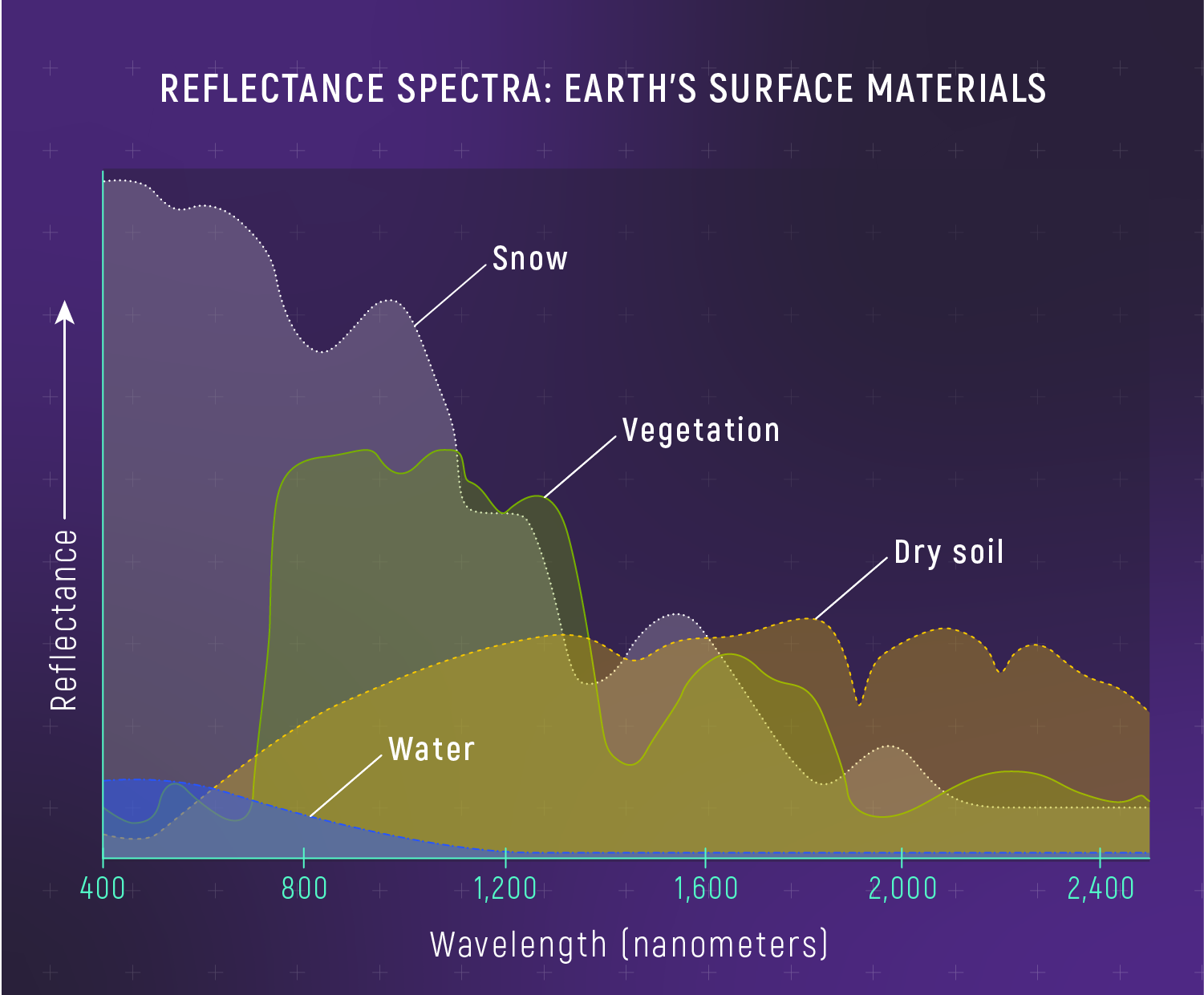
The physics has been understood since John Tyndall’s experiments (1861) and Svante Arrhenius’s calculations (1896): CO₂ absorbs infrared at specific wavelengths set by its molecular energy levels — the same quantum mechanics that produces hydrogen Balmer lines. Adding CO₂ to the atmosphere is, spectroscopically, equivalent to adding more absorbing atoms to a stellar atmosphere: the absorption features deepen.
Part 6 takeaway: the greenhouse effect is Kirchhoff’s third law applied to a planet — atmospheric molecules absorb infrared from the warm surface at specific wavelengths set by quantum mechanics. CO₂’s strong 15 μm band sits squarely in Earth’s thermal emission window. Increasing CO₂ deepens this absorption, traps more outgoing radiation, and warms the surface. The same spectroscopy that tells us what stars are made of tells us why our planet is warming.
Assumptions and Synthesis
Part 7: Assumptions and Limitations
Spectral classification assumes a single star. Unresolved binaries blend two spectra, complicating classification. Spectroscopic binaries are identified by two sets of absorption lines (double-lined) or periodic velocity oscillations (single-lined) — Lecture 4’s territory.
The Bohr model is approximate. It works beautifully for hydrogen but breaks down for multi-electron atoms, which need full quantum mechanics. The concept — discrete levels producing discrete lines — remains exactly right.
Line identification requires lab data. We match stellar lines to laboratory-measured wavelengths. If an element’s spectrum hasn’t been measured in the lab, we can’t identify it in a star. Historically, helium was found in the Sun’s spectrum before it was found on Earth — its lines matched no known element, so it was named for the Greek sun god (Helios).
Interstellar absorption adds extra lines. Gas and dust between us and a star imprint additional features (interstellar sodium D lines, diffuse interstellar bands). These are separated from the star’s own lines by checking whether they share the star’s Doppler shift (interstellar lines have their own, different velocity).
Part 7 takeaway: spectroscopy is robust but not foolproof. Binaries blend spectra, interstellar gas adds false lines, and precise composition requires careful modeling. These caveats don’t undermine the method — they refine it.
Summary: Observable → Model → Inference
| We observe | We use | We infer |
|---|---|---|
| Dark lines at specific wavelengths | Atomic physics: each element has unique energy levels (Bohr model) | Composition — which atoms are present |
| Relative strengths of different species’ lines | Boltzmann distribution: temperature controls level populations | Temperature and spectral type (OBAFGKM) |
| Lines shifted from lab wavelengths | Doppler formula | Radial velocity — motion toward/away |
| Width and shape of lines | Pressure broadening, rotation, turbulence | Atmospheric density, rotation, magnetic fields |
| Molecular bands in planetary spectra | Quantum mechanics of molecular vibrations | Atmospheric composition and greenhouse effect |
A star’s spectral lines are all shifted to slightly longer wavelengths by the same fractional amount. What does this tell you — and what does it not tell you about the star’s motion?
All lines shifting by the same fraction means a real Doppler shift: the star is receding (redshift), with . It does not tell you the star’s transverse (sideways) motion — that produces no shift and needs astrometry — nor its rotation, which broadens lines rather than shifting their centers.
Self-Assessment Checklist
After working through this reading, you should be able to:
- ☐ Sketch the three types of spectra and explain when each appears (Kirchhoff’s laws)
- ☐ Explain why stars show absorption spectra using the two-layer model (photosphere + atmosphere)
- ☐ Use the Bohr model to explain why spectral lines occur at specific wavelengths
- ☐ Calculate the wavelength of a hydrogen transition from energy levels
- ☐ Recite the OBAFGKM sequence and explain it as a temperature sequence
- ☐ Explain why H Balmer lines peak in strength at A-type temperatures
- ☐ Apply the Doppler formula to compute radial velocity from a line shift
- ☐ Distinguish spectral type, luminosity class, and metallicity
- ☐ Explain the greenhouse effect using Kirchhoff’s laws and molecular absorption bands
- ☐ Calculate a planet’s equilibrium temperature using Stefan-Boltzmann
Key Equations Reference
| Equation | Use | Notes |
|---|---|---|
| Hydrogen energy levels (Bohr model) | ; negative = bound | |
| Photon energy from wavelength | Connects quantum levels to spectral lines | |
| Wavelength of a spectral line | = energy gap between levels | |
| Doppler shift (non-relativistic) | receding (redshift); approaching (blueshift) | |
| fraction in level | Boltzmann distribution (qualitative) | = excitation energy above ground state; explains spectral type = temperature |
| Planetary equilibrium temperature | No greenhouse; bare energy balance | |
| Solar-system shortcut | For planets orbiting the Sun |
Key Constants
| Constant | Value | Units |
|---|---|---|
| Planck’s constant | erg·s | |
| Speed of light | cm/s ( km/s) | |
| Boltzmann’s constant | eV/K | |
| Stefan-Boltzmann constant | erg cm⁻² s⁻¹ K⁻⁴ | |
| Wien’s constant | nm·K | |
| Hydrogen ionization energy | 13.6 | eV |
| erg | ||
| Solar luminosity | erg/s | |
| cm |
Glossary
- Absorption line
A dark feature in a spectrum where a cool gas absorbs photons from a hotter background source at a specific wavelength set by an atomic energy-level gap. It appears at the same wavelength the gas would emit if heated.
- Albedo
The fraction of incident light a surface or planet reflects rather than absorbs. is perfect absorption; is a perfect mirror. The Moon has , Earth , Venus . Only the absorbed fraction heats the planet.
- Balmer series
Hydrogen spectral lines from transitions to or from the level. The visible members are Hα (656 nm), Hβ (486 nm), Hγ (434 nm), and Hδ (410 nm) — the most prominent features in many stellar spectra.
- Blueshift
A shift of spectral lines to shorter wavelengths (), indicating the source is approaching the observer.
- Bohr model
A quantum model of hydrogen in which the electron occupies discrete energy levels and absorbs or emits a photon only when it transitions between levels. Approximate for multi-electron atoms, but the core idea — discrete levels yield discrete lines — is exactly right.
- Boltzmann distribution
The rule that the fraction of atoms in an excited level scales as , where is the excitation energy above the ground state. Its exponential sensitivity to temperature is why spectral type is a temperature sequence: temperature, not abundance, sets which levels are populated and therefore which lines appear.
- Doppler shift
The change in observed wavelength caused by a source’s motion along the line of sight: . Receding sources shift to longer wavelengths (redshift); approaching sources shift to shorter wavelengths (blueshift).
- Equilibrium temperature
The temperature at which a planet radiates exactly as much energy as it absorbs from its star, assuming no atmosphere: . The greenhouse effect raises the real surface temperature above this baseline.
- Greenhouse effect
Warming of a planet’s surface caused by atmospheric gases absorbing outgoing infrared radiation and re-emitting part of it back downward. It is Kirchhoff’s third law applied to a planet: a cool atmosphere absorbing from the warm surface continuum.
- Kirchhoff's laws
Three rules linking the appearance of a spectrum to the physical conditions of its source: (1) a hot dense object yields a continuous spectrum; (2) a hot low-density gas yields bright emission lines; (3) a cool gas in front of a hotter continuum yields dark absorption lines at the same wavelengths it would emit. Worked backward, a spectrum’s appearance reveals the source’s configuration.
- Metallicity
The mass fraction of elements heavier than helium in a star or gas cloud (). It modulates the strength of metal absorption lines but, at fixed temperature, does not change a star’s spectral type — a second-order effect.
- Photosphere
The visible “surface” of a star — the depth at which it becomes opaque (optical depth ) and from which the continuous spectrum escapes. For the Sun it sits near 5,800 K; the slightly cooler atmosphere just above it carves the absorption lines.
- Radial velocity
The component of a star’s velocity along the observer’s line of sight, measured from the Doppler shift of its spectral lines. The perpendicular (transverse) motion produces no shift and must be measured astrometrically.
- Redshift
A shift of spectral lines to longer wavelengths (), indicating the source is receding from the observer.
- Spectrum
The intensity of light as a function of wavelength, obtained by dispersing light through a prism or diffraction grating. A spectrum is quantitative data: its continuum slope, emission peaks, and absorption lines each encode physical conditions of the source.