Decoding Starlight — Spectral Lines and Chemical Fingerprints
Lecture 9 Reading Companion
The Big Idea
Blackbody radiation tells us temperature. But real stellar spectra have something more: spectral lines — bright or dark features at specific wavelengths. These lines are chemical fingerprints, revealing what stars are made of. Each element has its own unique pattern, and quantum mechanics explains why.
This reading covers spectral lines, the quantum origin of discrete spectra, and stellar classification — the foundation for understanding stellar composition.
Structure:
- Part 1: Spectral lines and what causes them (Kirchhoff’s Laws)
- Part 2: Quantum mechanics (conceptual) — why energy is quantized
- Part 3: Stellar classification (OBAFGKM) and HR diagram preview
Musts for today (~35-45 min):
- The Big Idea
- Kirchhoff’s Three Laws
- Why spectral lines are discrete (quantized energy levels)
- Hydrogen energy levels deep dive
- OBAFGKM classification and why hydrogen lines peak at A stars
Non-negotiable: Stop at every Check Yourself question — don’t just read past them!
What’s next: In L10 (Friday), we’ll learn how these same spectral lines reveal motion through the Doppler effect — and how telescopes collect this light.
If you only remember three things:
Each element has a unique fingerprint. Hydrogen absorbs at 656 nm, 486 nm, 434 nm… No other element produces this exact pattern.
Lines are discrete because energy is quantized. Electrons can only occupy specific energy levels in atoms — like rungs on a ladder, not a ramp.
OBAFGKM orders stars by temperature. O is hottest (blue), M is coolest (red). Hydrogen lines are strongest in A stars — not because they have more hydrogen, but because of temperature and ionization physics.
Now for the details…
The Missing Colors
In 1814, German optician Joseph von Fraunhofer pointed a prism at sunlight and made a puzzling discovery. The rainbow spectrum wasn’t smooth — it was crossed by hundreds of dark lines, specific wavelengths where light was missing. He catalogued over 500 of them, labeling many prominent lines with letters (A, B, C, D, …).
Fraunhofer didn’t know what caused these lines. But by the 1860s, Gustav Kirchhoff and Robert Bunsen had cracked the code: each chemical element absorbs and emits light at specific wavelengths. The dark lines in the solar spectrum are wavelengths absorbed by elements in the Sun’s outer atmosphere. The pattern of lines is a chemical fingerprint.
This was revolutionary. For the first time, humans could determine what a star is made of — without touching it, without visiting it, from 150 million kilometers away. And once we understood the physics, we realized: these same lines could reveal motion (via Doppler shifts — that’s L10!), magnetic fields, pressure, and more.
In Lectures 7 and 8, we learned that light carries information: wavelength, intensity, temperature. Now we add another layer: spectral lines tell us composition. By the end of this lecture, you’ll understand why each element has a unique fingerprint and how astronomers use this to classify stars.
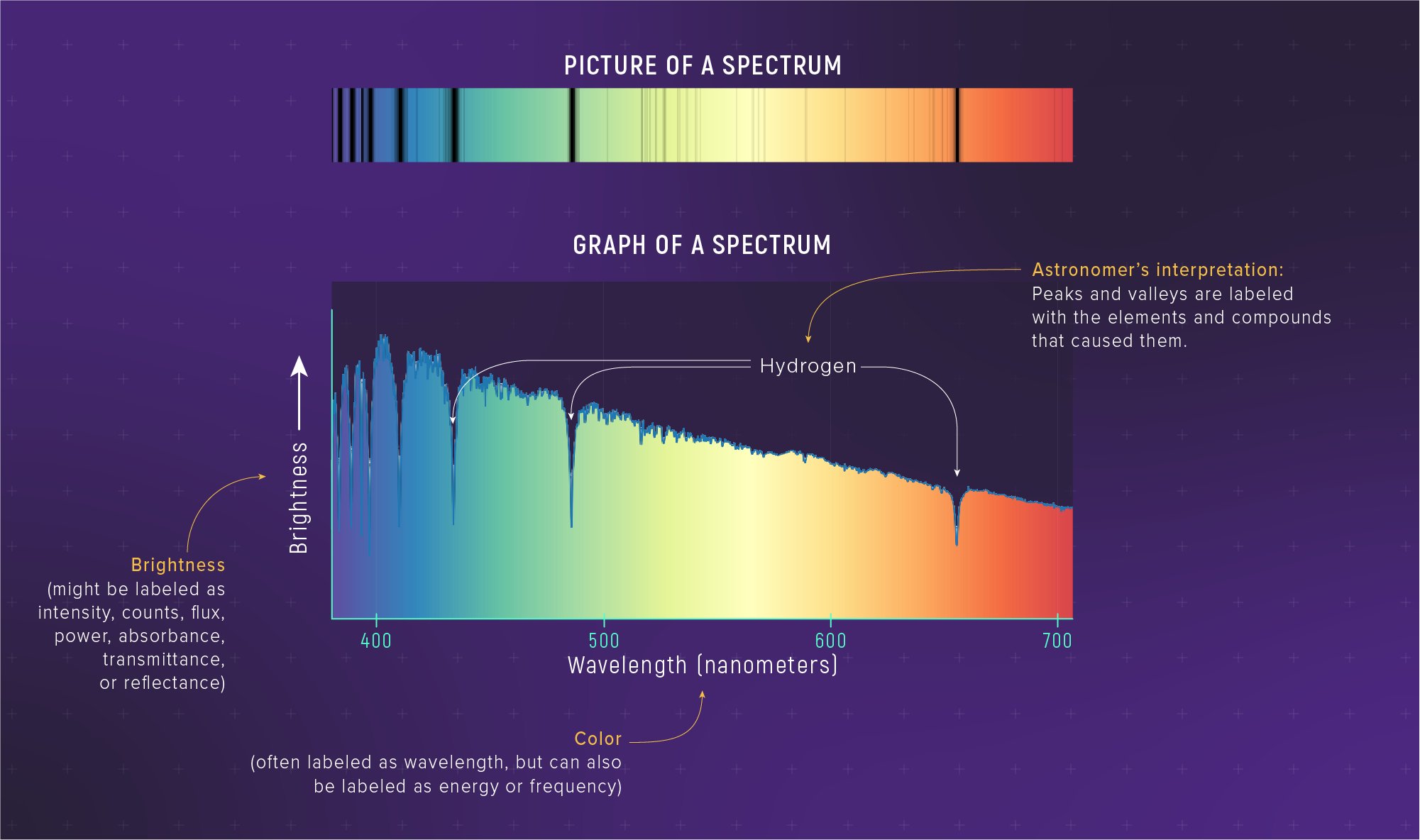
What to notice: a spectrum can be shown as both an image (colored strip) and a graph; the dips and features are where atoms absorb light. (Credit: Illustration: NASA, ESA, CSA)
In Lecture 8, we discovered how temperature is written in light:
- Blackbody radiation: hot objects glow, with spectrum determined by temperature
- Wien’s Law: peak wavelength tells temperature (\(\lambda_{peak} \propto 1/T\))
- Stefan-Boltzmann: luminosity depends powerfully on temperature (\(L \propto T^4\))
But we noted that real stellar spectra aren’t perfect blackbodies — they have lines. Now we explore where those lines come from and what they tell us.
The key insight: Blackbody gives temperature. Spectral lines give composition.
Part 1: Three Types of Spectra
Kirchhoff’s Discovery
In the 1860s, Kirchhoff discovered three rules that predict what kind of spectrum you’ll see, depending on the physical conditions. These became the foundation of spectroscopy — the science of reading light.
1. Continuous Spectrum (Blackbody) A hot, dense object (solid, liquid, or dense gas) emits light at all wavelengths — a smooth rainbow with no gaps.
2. Emission Spectrum (Bright Lines) A hot, thin (low-density) gas emits light at specific wavelengths only — bright lines on a dark background.
3. Absorption Spectrum (Dark Lines) A cool gas in front of a hot, continuous source absorbs light at specific wavelengths — dark lines on a bright rainbow background.
Continuous spectrum: A smooth spectrum containing all wavelengths, like a rainbow. Produced by hot, dense objects.
Emission spectrum: Bright lines at specific wavelengths on a dark background. Produced by hot, thin gas.
Absorption spectrum: Dark lines at specific wavelengths on a continuous background. Produced when cool gas sits in front of a hot source.
🔭 Demo Exploration: Spectral Lines Lab
Open the Spectral Lines Lab demo: ../../../demos/spectral-lines-lab/
This demo lets you switch physical setups (Kirchhoff’s laws) and practice identifying elements by line patterns, not single lines.
Mission A (Kirchhoff)
Predict before you click: Which setup produces an absorption spectrum?
Write your prediction here: _______________
Mission B (fingerprints)
Turn on the unknown spectrum overlay. Your goal is to find the element set that matches the unknown by pattern matching.
Mission C (mixtures)
Explain in one sentence: “Why does the Sun have a continuous spectrum and absorption lines?”
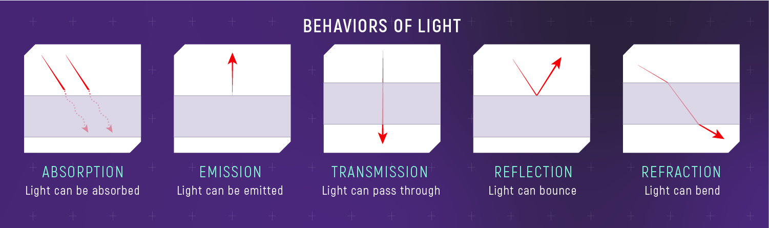
What to notice: light can be absorbed, emitted, transmitted, reflected, or refracted—those interactions are how spectra are made. (Credit: Illustration: NASA, ESA, CSA)
Visual Summary
Picture three scenarios:
A hot filament in a light bulb: Dense, glowing metal \(\rightarrow\) smooth, continuous rainbow spectrum
A neon sign: Hot, thin neon gas \(\rightarrow\) bright red-orange lines on a dark background
The Sun: Hot interior (continuous spectrum) + cooler outer atmosphere (absorbs specific wavelengths) \(\rightarrow\) continuous spectrum with dark lines
The third scenario is exactly what creates the Fraunhofer lines. The Sun’s photosphere produces a continuous blackbody-like spectrum. As that light passes through the cooler layers above it, atoms absorb light at their characteristic wavelengths, creating dark absorption lines.
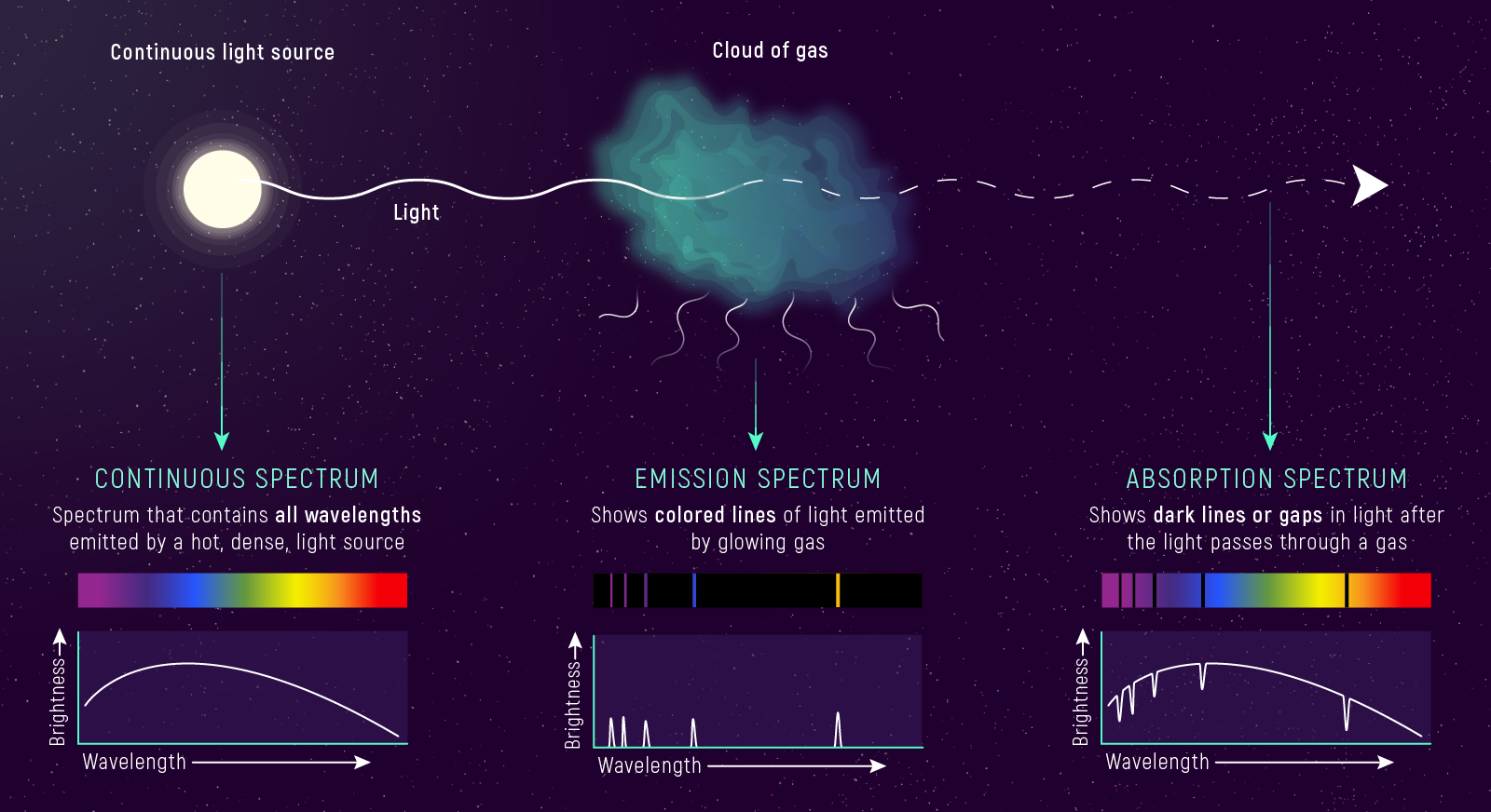
What to notice: continuous, emission-line, and absorption-line spectra come from different physical setups (Kirchhoff’s three laws). (Credit: Illustration: NASA, ESA, CSA)
Why This Matters for Stars
Every star works like the Sun in this regard:
- Hot interior: Dense \(\rightarrow\) continuous blackbody spectrum
- Cooler outer atmosphere: Thin gas \(\rightarrow\) absorption at specific wavelengths
- What we see: Continuous spectrum crossed by dark absorption lines
The pattern of dark lines tells us which elements are in the star’s atmosphere. Each element has a unique pattern — a chemical barcode. Read the barcode, identify the elements.
The dark lines in the Sun’s spectrum are caused by:
- The Sun’s core being too cool to emit those wavelengths
- Cool gas in the Sun’s outer atmosphere absorbing specific wavelengths
- Earth’s atmosphere blocking the light
- The Sun rotating and shifting the wavelengths
B) Cool gas in the Sun’s outer atmosphere absorbing specific wavelengths.
The Sun’s photosphere produces a continuous spectrum. As that light passes through the cooler layers above it, atoms absorb light at their characteristic wavelengths, creating dark absorption lines. (Earth’s atmosphere does add some lines, but the Fraunhofer lines are solar in origin.)
Each Element Has a Unique Pattern
Chemical Fingerprints
Every element — hydrogen, helium, carbon, iron — absorbs and emits light at a unique set of wavelengths. This pattern is as distinctive as a fingerprint or barcode.
- Hydrogen: Strong lines at 656 nm (red), 486 nm (blue-green), 434 nm (violet)…
- Sodium: Bright yellow doublet at 589 nm (the famous “D lines”)
- Calcium: Strong lines in the violet (H and K lines at 397 and 393 nm)
- Iron: Hundreds of lines throughout the visible spectrum
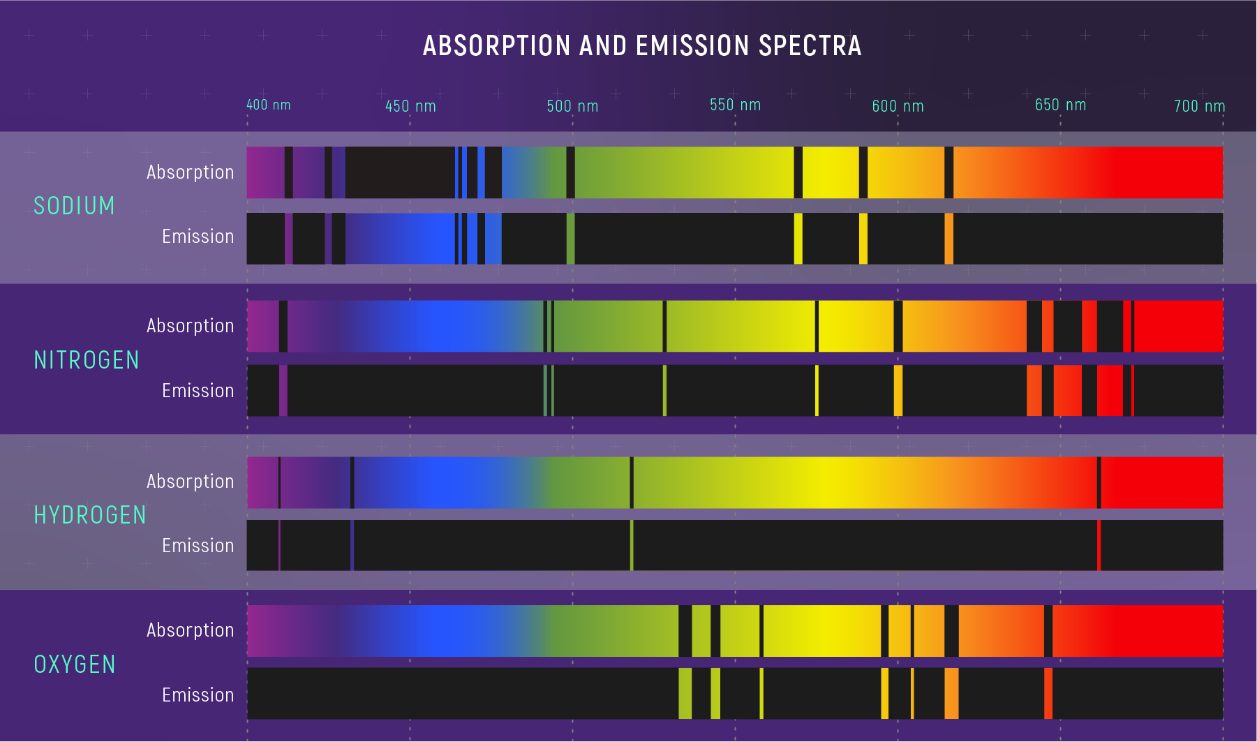
What to notice: absorption and emission lines occur at the same wavelengths for a given element—same atomic fingerprints, seen in opposite ways. (Credit: Illustration: NASA, ESA, CSA)
Spectral line: A bright or dark feature at a specific wavelength, caused by emission or absorption by atoms. Each element has its own unique set of lines.
How We Identify Elements
To identify elements in a star:
- Observe the star’s spectrum
- Measure the wavelengths of absorption lines
- Compare to laboratory measurements of known elements
- Match the pattern \(\rightarrow\) identify the element
This is how we know the Sun is ~74% hydrogen, ~24% helium, and ~2% heavier elements by mass (“metals” in astronomy jargon) — without ever collecting a sample.
Observable: The Sun’s spectrum shows absorption lines at 656.28 nm, 486.13 nm, 434.05 nm (and many more). Dark lines also appear at 589 nm (sodium) and 393/397 nm (calcium).
Model: Each element produces absorption at specific wavelengths. Laboratory measurements give us the reference patterns.
Inference: The Sun’s atmosphere contains hydrogen, sodium, calcium, and many other elements. By measuring line strengths, we can estimate relative abundances.
In 1868, astronomers observing a solar eclipse noticed an emission line at 587.6 nm that didn’t match any known element on Earth. They named the mystery element helium — from helios, the Greek word for Sun.
Helium wasn’t isolated on Earth until 1895, nearly 30 years later. Spectroscopy revealed a new element 150 million km away before we found it in our own laboratories!
This remains one of astronomy’s most remarkable achievements: discovering an element through starlight before finding it on our own planet.
How do astronomers determine which elements are present in a star?
- By measuring the star’s temperature
- By matching the pattern of spectral lines to laboratory measurements
- By observing the star’s color
- By measuring how bright the star is
B) By matching the pattern of spectral lines to laboratory measurements.
Each element produces a unique pattern of absorption or emission lines. By comparing observed stellar spectra to lab spectra of known elements, astronomers identify which elements are present. Temperature affects which lines are visible (more on that soon), but the identification comes from pattern matching.
Part 2: The Quantum Origin of Spectral Lines
The Puzzle of Discrete Lines
Here’s a puzzle: if atoms can absorb and emit light, why only at specific wavelengths? Why not a continuous range?
Before 1913, this was a mystery. Classical physics predicted that atoms should emit light at all wavelengths — electrons could have any energy, so any wavelength should be possible. But that’s not what we observe. Spectral lines are sharp and discrete. Something deeper was going on.
The Breakthrough: Energy Is Quantized
The answer came from quantum mechanics: energy in atoms isn’t continuous — it’s quantized. Electrons can only occupy specific energy levels, like rungs on a ladder. They can’t exist between rungs.
Quantized: Restricted to specific discrete values, not continuous. Like steps on a staircase, not a ramp.
Energy level: A specific, allowed energy state for an electron in an atom.
Ground state: The lowest energy level an electron can occupy.
Excited state: Any energy level higher than the ground state.
The Ladder Analogy
Imagine a ladder where you can only stand on the rungs, never between them. Electrons in atoms are like this — they can only occupy specific energy levels.
To move from one rung to another, the electron must gain or lose exactly the right amount of energy. That energy comes from (or goes into) a photon.
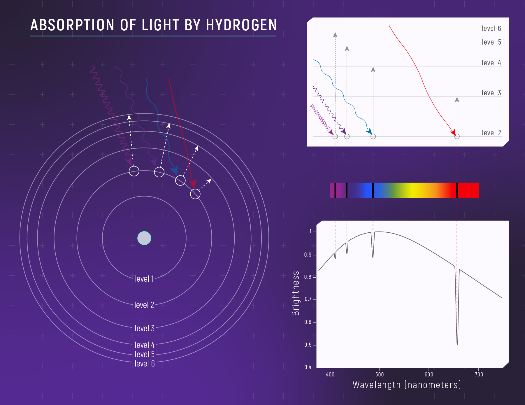
What to notice: when cooler hydrogen gas sits in front of a hotter source, it absorbs specific wavelengths—creating dark absorption lines. (Credit: Illustration: NASA, ESA, CSA)
Classical assumption: Energy can vary continuously, like a ramp. An electron could have any energy, and atoms could emit any wavelength.
Quantum reality: Energy is quantized, like a staircase. Only specific energy values are allowed, so only specific wavelengths appear.
This was one of the most profound discoveries of the 20th century: at atomic scales, nature is fundamentally discrete, not continuous.
Photons and Energy Transitions
The Photon-Energy Connection
When an electron jumps between energy levels:
- Absorption: Electron jumps UP to higher energy level. A photon with exactly the right energy is absorbed.
- Emission: Electron jumps DOWN to lower energy level. A photon with exactly that energy is emitted.
\[ E_{photon} = h\nu = \frac{hc}{\lambda} \]
where:
- \(h = 6.63 \times 10^{-34}\) \(J\cdot s\) (Planck’s constant)
- \(\nu\) = frequency of the light
- \(\lambda\) = wavelength of the light
- \(c\) = speed of light
Higher energy photon \(\leftrightarrow\) higher frequency \(\leftrightarrow\) shorter wavelength
Why Lines Are Discrete
The photon energy must exactly match the energy gap between two levels:
\[ E_{photon} = E_{upper} - E_{lower} \]
Since atoms have only specific allowed energy levels, they can only absorb/emit photons with specific energies — which means specific wavelengths. That’s why spectral lines are sharp and discrete, not blurry or continuous.
Think of it like a vending machine that only accepts exact change. You can’t insert any amount — only the specific denominations that match the price. Atoms are similar: they only “accept” photons with exactly the right energy to move an electron between levels.
Deep Dive: Hydrogen Energy Levels
Why Hydrogen?
Hydrogen is the simplest atom: one proton, one electron. Its energy levels can be calculated exactly, and the formula is elegant.
We focus on hydrogen because it’s the simplest case — and the only atom where the energy levels follow a single, elegant formula. Think of this as training wheels for understanding spectral lines.
Real atoms are more complex: Helium has two electrons that interact with each other. Iron has 26. Their energy levels don’t follow a simple formula, and they produce hundreds or thousands of lines each.
But the principle is the same: quantized energy levels \(\rightarrow\) discrete spectral lines. Once you understand hydrogen, you have the conceptual foundation for all atomic spectroscopy.
\[ E_n = -\frac{13.6 \text{ eV}}{n^2} \quad (n = 1, 2, 3,...) \]
where:
- \(n\) = principal quantum number (1, 2, 3, …)
- \(E_n\) = energy of level \(n\)
- The negative sign means the electron is bound to the atom
- \(n = \infty\) corresponds to \(E = 0\) (electron freed/ionized)
Electron volt (eV): A convenient energy unit for atoms. 1 eV = \(1.6 \times 10^{-19}\) J. Visible photons have energies of about 1.8–3.1 eV.
Principal quantum number (n): An integer (1, 2, 3, …) that labels the energy levels of hydrogen. Higher n = higher energy (less negative).
The Energy Level Diagram
Let’s calculate some energy levels:
| Level (\(n\)) | Calculation | Energy (\(E_n\)) | Name |
|---|---|---|---|
| 1 | \(-13.6/1^2\) | -13.6 eV | Ground state |
| 2 | \(-13.6/2^2\) | -3.4 eV | First excited state |
| 3 | \(-13.6/3^2\) | -1.51 eV | Second excited state |
| 4 | \(-13.6/4^2\) | -0.85 eV | Third excited state |
| ∞ | \(-13.6/\infty^2\) | 0 eV | Ionized (free electron) |
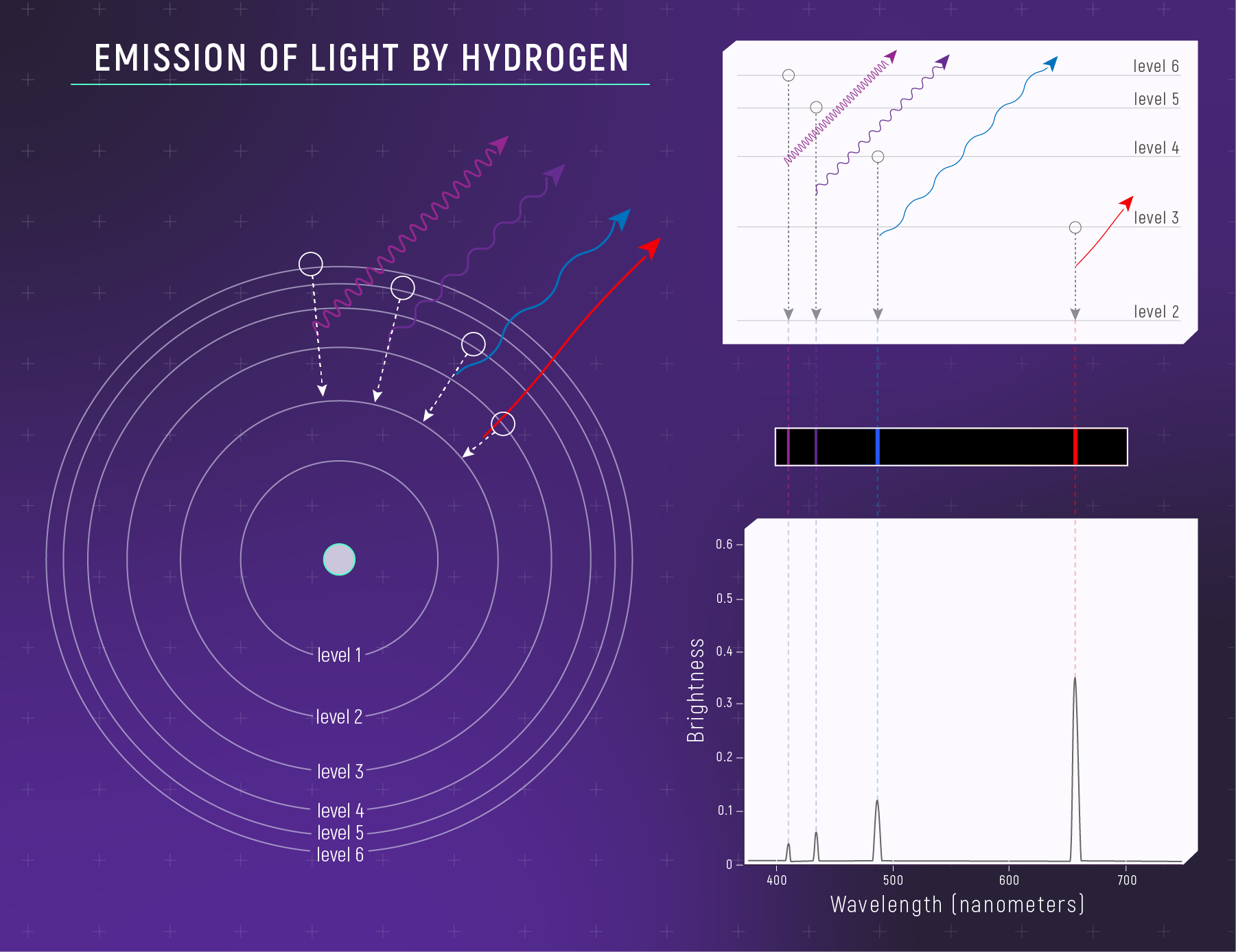
What to notice: a hot, low-density hydrogen gas emits light at specific wavelengths—creating bright emission lines. (Credit: Illustration: NASA, ESA, CSA)
Notice that the levels get closer together as \(n\) increases. This is because of the \(1/n^2\) dependence — a characteristic signature of hydrogen.
The Balmer Series (Visible Lines)
Transitions that end at n = 2 produce visible light — the Balmer series:
| Transition | Energy Released | Wavelength | Color | Name |
|---|---|---|---|---|
| 3 \(\rightarrow\) 2 | 1.89 eV | 656 nm | Red | \(H\alpha\) (H-alpha) |
| 4 \(\rightarrow\) 2 | 2.55 eV | 486 nm | Blue-green | \(H\beta\) (H-beta) |
| 5 \(\rightarrow\) 2 | 2.86 eV | 434 nm | Violet | \(H\gamma\) (H-gamma) |
| 6 \(\rightarrow\) 2 | 3.02 eV | 410 nm | Violet | \(H\delta\) (H-delta) |
Balmer series: The set of hydrogen spectral lines from transitions ending at n=2. These are visible light lines, named \(H\alpha,\) \(H\beta,\) \(H\gamma,\) \(H\delta,\) etc.
Worked Example: Calculating \(H\alpha\) Wavelength
Problem: Calculate the wavelength of light emitted when a hydrogen electron drops from n=3 to n=2.
Solution:
Step 1: Find the energies of each level \[ E_3 = -\frac{13.6}{3^2} = -\frac{13.6}{9} = -1.51 \text{ eV} \] \[ E_2 = -\frac{13.6}{2^2} = -\frac{13.6}{4} = -3.4 \text{ eV} \]
Step 2: Find the energy difference (photon energy) \[ E_{photon} = E_3 - E_2 = -1.51 - (-3.4) = 1.89 \text{ eV} \]
Step 3: Convert to wavelength using \(E = hc/\lambda\)
Using the convenient shortcut: \(\lambda \text{ (nm)} = \frac{1240 \text{ eV\cdot nm}}{E \text{ (eV)}}\) \[ \lambda = \frac{1240}{1.89} = 656 \text{ nm} \]
This is \(H\alpha\) — the famous red hydrogen line! It’s the brightest line in many emission nebulae and the reason hydrogen nebulae glow reddish-pink.
The “1240” shortcut comes from combining fundamental constants:
\[ \lambda = \frac{hc}{E} = \frac{(6.63 \times 10^{-34} \text{ J\cdot s})(3 \times 10^8 \text{ m/s})}{E} \]
When you convert joules to eV and meters to nanometers, it simplifies to:
\[ \lambda \text{ (nm)} = \frac{1240}{E \text{ (eV)}} \]
This is a handy formula for atomic physics — memorize it once and save yourself many calculations!
Why This Matters
This single formula (\(E_n = -13.6/n^2\) eV) predicts the wavelengths of hydrogen lines to extraordinary precision. When astronomers observe a star and see absorption at exactly 656.28 nm, 486.13 nm, 434.05 nm… they know hydrogen is present.
Each element has its own energy level structure (more complex than hydrogen), producing its own unique line pattern. Quantum mechanics explains why spectral lines exist and predicts exactly where they’ll appear.
Which transition produces the shortest wavelength (highest energy) photon?
- n = 2 \(\rightarrow\) n = 1
- n = 3 \(\rightarrow\) n = 2
- n = 4 \(\rightarrow\) n = 3
- n = 5 \(\rightarrow\) n = 4
A) n = 2 \(\rightarrow\) n = 1. This transition has the largest energy gap:
\(|E_1 - E_2| = |{-13.6} - ({-3.4})| = 13.6 - 3.4 = 10.2\) eV
Larger energy gap = higher energy photon = shorter wavelength. (This is the Lyman-alpha line at 121.6 nm, in the ultraviolet — the brightest line in the far-UV sky.)
Spectral lines are discrete (specific wavelengths only) because:
- Telescopes can only detect certain wavelengths
- Atoms can only absorb red, green, and blue light
- Electrons in atoms can only occupy specific quantized energy levels
- Light travels at a constant speed
C) Electrons in atoms can only occupy specific quantized energy levels.
Photons are absorbed or emitted only when their energy exactly matches the gap between two allowed levels. Discrete levels \(\rightarrow\) discrete photon energies \(\rightarrow\) discrete wavelengths. This is quantum mechanics in action!
Part 3: Stellar Classification
The OBAFGKM Sequence
Classifying Stars by Spectra
When astronomers began systematically classifying stellar spectra in the late 1800s, they noticed that stars grouped into categories based on the strength of various absorption lines. Originally the classes were labeled alphabetically by hydrogen line strength. After much sorting and re-sorting (and realizing the pattern was really about temperature), the modern sequence emerged:

What to notice: the women of the Harvard Observatory — including Williamina Fleming, Annie Jump Cannon, and Cecilia Payne — classified hundreds of thousands of stellar spectra by hand, creating the system we still use today. (Credit: Harvard College Observatory)
Much of this monumental classification work was done by the “Harvard Computers” — women astronomers at Harvard College Observatory including Williamina Fleming, Annie Jump Cannon, and Cecilia Payne-Gaposchkin. Cannon personally classified over 350,000 stellar spectra, and Payne-Gaposchkin’s 1925 thesis demonstrated that stars are made primarily of hydrogen and helium — one of the most important results in 20th-century astrophysics.
O - B - A - F - G - K - M
This sequence orders stars by surface temperature, from hottest (O) to coolest (M).
Spectral type: A classification of stars based on their absorption line patterns, which correlates with surface temperature. O is hottest, M is coolest.
The Spectral Types
| Type | Color | Temperature (K) | Prominent Features | Example Stars |
|---|---|---|---|---|
| O | Blue | 30,000–50,000+ | Ionized helium, weak hydrogen | Mintaka, Alnitak |
| B | Blue-white | 10,000–30,000 | Neutral helium, moderate hydrogen | Rigel, Spica |
| A | White | 7,500–10,000 | Strongest hydrogen (Balmer) | Sirius, Vega |
| F | Yellow-white | 6,000–7,500 | Hydrogen, ionized metals | Procyon, Canopus |
| G | Yellow | 5,000–6,000 | Calcium, iron lines | The Sun, Alpha Centauri A |
| K | Orange | 3,500–5,000 | Strong metal lines | Arcturus, Aldebaran |
| M | Red | 2,500–3,500 | Molecular bands (TiO) | Betelgeuse, Proxima Centauri |
Classic mnemonic: “Oh Be A Fine Girl/Guy, Kiss Me”
(Or if you prefer: “Only Brilliant Astronomers Figure Galactic Kinematics Meaningfully”)
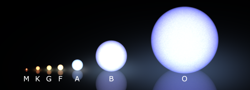
What to notice: the Morgan–Keenan system classifies stars by spectral type (O through M) and luminosity class. Hotter stars are bluer and more luminous; cooler stars are redder and dimmer. Size differences between giants and dwarfs are dramatic. (Credit: Wikimedia Commons (public domain))
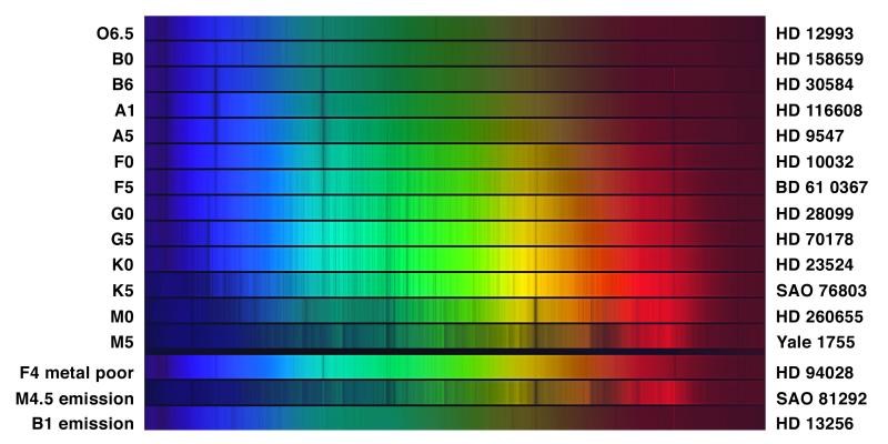
What to notice: real stellar spectra change dramatically across spectral types. Hot O stars show few lines (ionized gas); A stars show strong hydrogen Balmer lines; cool M stars show broad molecular absorption bands. The pattern reflects temperature, not composition. (Credit: NOAO/AURA/NSF)
Each spectral type is subdivided 0–9, from hottest to coolest within the class. The Sun is a G2 star (toward the hot end of G). Vega is A0 (hottest A star). This gives astronomers finer temperature resolution.
Why Hydrogen Lines Peak at A Stars
Here’s a puzzle: hydrogen is the most abundant element in the universe (about 75% by mass), yet hydrogen lines are strongest in A stars (around 10,000 K), not in the hottest O stars. Why?
The answer involves temperature and ionization:
Too hot (O, B stars): At temperatures above ~15,000 K, hydrogen is mostly ionized — the electron is stripped away entirely. No bound electron = no absorption lines. The hydrogen is there, but it can’t produce visible absorption.
Too cool (K, M stars): At temperatures below ~5,000 K, most hydrogen electrons are in the ground state (n=1). To absorb Balmer-series light (visible wavelengths), the electron must already be in n=2 (an excited state). At low temperatures, few electrons are excited to n=2, so Balmer absorption is weak.
Just right (A stars ~10,000 K): Hydrogen is mostly neutral (not ionized), AND there’s enough thermal energy to excite electrons into n=2. Maximum Balmer absorption!
This is a beautiful example of physics: the strength of spectral lines depends not just on abundance but on temperature and ionization state. A star with weak hydrogen lines isn’t necessarily hydrogen-poor — it might just be too hot or too cool for hydrogen to produce visible absorption.
Intuitive assumption: Stronger lines = more of that element present.
Reality: Line strength depends on temperature and ionization, not just abundance. An O star has as much hydrogen as an A star, but you can’t see it in visible absorption because the hydrogen is ionized.
This is why spectral classification was so confusing before physicists understood atomic structure!
Which spectral type corresponds to the hottest stars?
- M
- G
- A
- O
D) O. The sequence OBAFGKM runs from hottest to coolest. O stars have temperatures above 30,000 K — they appear blue and have short lifetimes because they burn through fuel so fast. (M stars are the coolest, below 3,500 K — they appear red and can live for trillions of years.)
Hydrogen absorption lines are weak in O-type stars because:
- O stars contain very little hydrogen
- O stars are so hot that hydrogen is mostly ionized
- O stars are too cool to excite hydrogen
- O stars have thick atmospheres that block hydrogen lines
B) O stars are so hot that hydrogen is mostly ionized.
At temperatures above ~15,000 K, hydrogen loses its electron and becomes ionized. No bound electron means no absorption lines. The hydrogen is abundant — you just can’t see it in visible spectral lines. This fooled early astronomers into thinking O stars were hydrogen-poor!
The HR Diagram — A Sneak Peek
What’s Coming in Module 2
In Module 2, we’ll combine everything we’ve learned: temperature (from spectra or color), luminosity (from brightness and distance), and the L-T-R relationship from L8. When you plot luminosity vs. temperature for thousands of stars, a remarkable pattern emerges: the Hertzsprung-Russell (H-R) diagram.
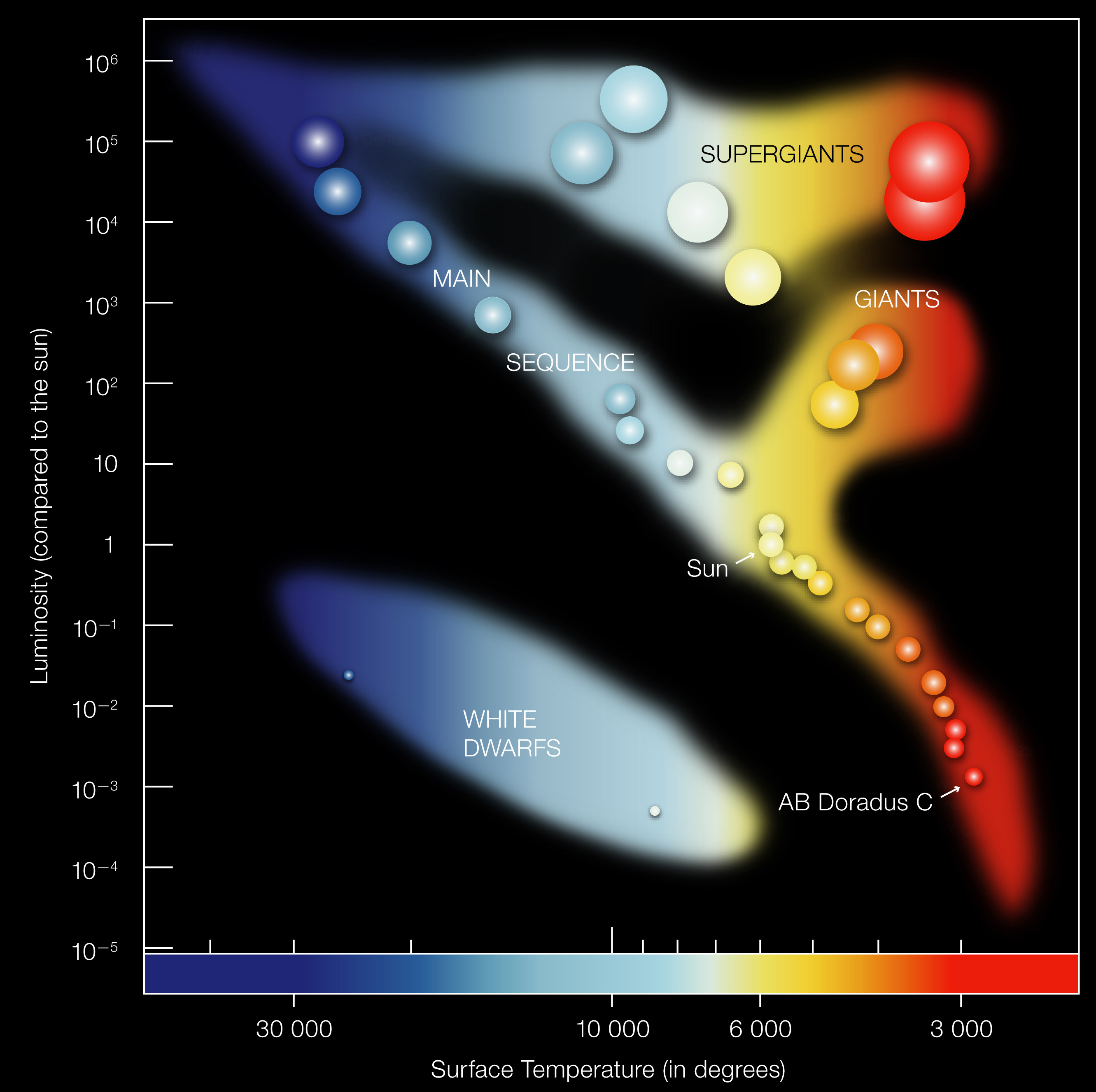
What to notice: the H-R diagram maps stars by temperature and luminosity; the main sequence, giants, and white dwarfs occupy distinct regions. (Credit: ESO)
This diagram is the astronomer’s periodic table — a map of stellar properties that reveals the physics of stellar structure and evolution. Every dot is a star. The patterns aren’t random — they reflect stellar physics.
Why the Patterns Exist
Main sequence: A diagonal band from upper-left (hot, luminous) to lower-right (cool, dim). These are stars fusing hydrogen in their cores — the “adult” phase of stellar life. A star’s position depends on its mass: more massive = hotter, more luminous.
Red giants: Upper-right region (cool but very luminous). These are stars that have exhausted core hydrogen and expanded enormously. Same temperature as small red dwarfs, but far more luminous = much larger radius. (Remember L-T-R from L8: same T, higher L \(\rightarrow\) larger R!)
White dwarfs: Lower-left region (hot but very dim). These are dead stellar cores — the leftover cores of stars that have shed their outer layers. Hot (still cooling down) but tiny = low luminosity.
In Module 2, we’ll trace stellar evolution across this diagram — from birth in molecular clouds to death as white dwarfs, neutron stars, or black holes.
With the physics from Module 1, you can now understand the HR diagram:
- Why giants are giant: Same T as dwarfs, higher L \(\rightarrow\) larger R (Stefan-Boltzmann from L8)
- Why O stars are at top-left: Hot \(\rightarrow\) blue (Wien’s Law), and massive \(\rightarrow\) luminous
- Why M dwarfs are at bottom-right: Cool \(\rightarrow\) red, and small \(\rightarrow\) dim
- Why the main sequence exists: Stars in hydrostatic equilibrium follow a mass-luminosity relation
Module 2 is where we apply these tools to understand stellar lives.
Spectral Lines:
Kirchhoff’s Laws: Hot dense \(\rightarrow\) continuous spectrum; hot thin gas \(\rightarrow\) emission lines; cool gas in front of hot source \(\rightarrow\) absorption lines
Each element has a unique fingerprint of spectral lines. Match the pattern \(\rightarrow\) identify the element.
Energy is quantized: Electrons occupy discrete levels, absorb/emit photons only at specific energies (wavelengths). This is why lines are sharp, not continuous.
Hydrogen: \(E_n = -13.6\text{ eV}/n^2\). Balmer series (transitions to n=2) gives visible lines at 656 nm, 486 nm, 434 nm…
OBAFGKM spectral types order stars from hot (O, blue) to cool (M, red). Hydrogen lines peak at A stars — not because of abundance, but because of ionization physics.
What’s Next:
In L10, we’ll see what happens when these spectral fingerprints shift — the Doppler effect reveals motion, from exoplanets to dark matter. And we’ll explore telescopes — the instruments that collect this light.
Self-Assessment Checklist
Before moving on, check your understanding. You should be able to do all of the following:
Kirchhoff’s Laws (Part 1):
Quantum Mechanics (Part 2):
Stellar Classification (Part 3):
If any box is unchecked, go back to that section and re-read it before attempting the practice problems.
Practice Problems
Solutions are available in the Lecture 9 Solutions.
Core (do these first)
1. Kirchhoff’s Laws (Conceptual): What type of spectrum (continuous, emission, or absorption) would you see from a hot, thin gas cloud with no background light source?
2. Hydrogen Levels (Calculation): Using \(E_n = -13.6/n^2\) eV, calculate the energy of a photon emitted when a hydrogen electron falls from n=4 to n=2. What color would this light be? (Use \(\lambda = 1240/E\) with E in eV to get wavelength in nm.)
3. Spectral Types (Application): A star shows very strong hydrogen Balmer lines but no helium lines. What spectral type is most likely? Is it hotter or cooler than the Sun?
4. Ionization and Lines (Conceptual): Explain in your own words why hydrogen absorption lines are weak in both O stars and M stars, even though both contain abundant hydrogen.
5. Line Identification (Application): A star’s spectrum shows strong absorption at 656 nm and 486 nm. What element is definitely present?
Challenge
6. Balmer Limit (Calculation): What is the shortest wavelength of the Balmer series (n=∞ \(\rightarrow\) 2)? In what part of the spectrum is this? (Hint: what’s the maximum energy a Balmer photon can have?)
7. Why Not Hotter? (Conceptual): Explain why hydrogen absorption lines are weaker in O stars than in A stars, even though O stars are hotter and hydrogen is the most abundant element.
8. Lyman Series (Calculation): The Lyman series consists of transitions to n=1. The Lyman-alpha line (n=2 \(\rightarrow\) 1) has a wavelength of 121.6 nm. In what part of the EM spectrum is this? Why can’t ground-based telescopes observe Lyman-alpha lines from stars?
Synthesis
9. Mystery Star (Synthesis): A star’s spectrum shows \(H\alpha\) absorption at 656 nm with no wavelength shift, strong calcium H and K lines (393 and 397 nm), many iron lines, but no helium lines. The hydrogen Balmer lines are moderate — not the strongest you’ve seen, but clearly present.
- What elements can you identify in this star’s atmosphere?
- What spectral type is most consistent with these features? Explain your reasoning using what you know about temperature and ionization.
- Using the Observable \(\rightarrow\) Model \(\rightarrow\) Inference framework, write a 2–3 sentence summary of what this spectrum tells us about the star.
(Hint: Think about which spectral type shows moderate hydrogen, strong calcium and iron, and no helium.)
Glossary
| Term | Definition |
|---|---|
| Spectral line | A bright or dark feature at a specific wavelength, caused by emission or absorption by atoms |
| Continuous spectrum | A smooth spectrum containing all wavelengths (like a blackbody) |
| Emission spectrum | Bright lines on a dark background, from a hot thin gas |
| Absorption spectrum | Dark lines on a bright background, from cool gas in front of a hot source |
| Quantized | Restricted to discrete values rather than continuous (like stair steps, not a ramp) |
| Energy level | A specific allowed energy state for an electron in an atom |
| Ground state | The lowest energy level of an electron (n=1 for hydrogen) |
| Excited state | Any energy level above the ground state |
| Balmer series | Hydrogen spectral lines from transitions ending at n=2 (visible light) |
| OBAFGKM | The stellar spectral classification sequence from hot to cool |
| Ionization | Removal of an electron from an atom |
- ★ Balmer series
- The set of hydrogen emission/absorption lines corresponding to transitions to/from the n=2 energy level. Includes Hα (656 nm, red), Hβ (486 nm, blue-green), Hγ (434 nm, violet).
- ★ Energy level
- A discrete allowed energy state for an electron in an atom; electrons can only occupy specific levels. Transitions between levels produce photons with specific energies (and wavelengths).
- ◇ Excited state
- Any energy level above the ground state; atoms in excited states tend to emit photons and drop to lower levels. An atom can be excited by absorbing a photon or through collisions.
- ◇ Ground state
- The lowest energy level of an atom; the n=1 level for hydrogen. Atoms 'prefer' the ground state; excited atoms quickly return to it.
- ★ Kirchhoff's First Law
- A hot, dense gas or solid produces a continuous spectrum (all wavelengths). Examples: the interior of a star, a glowing filament.
- ★ Kirchhoff's Second Law
- A hot, low-density gas produces an emission-line spectrum (bright lines at specific wavelengths). Examples: neon signs, nebulae.
- ★ Kirchhoff's Third Law
- A cool gas in front of a hot source produces an absorption-line spectrum (dark lines at specific wavelengths). This is what we see in stellar spectra—absorption lines from the cooler outer atmosphere.
- ★ OBAFGKM
- The spectral classification sequence for stars, ordered from hottest (O, ~40,000 K) to coolest (M, ~3,000 K). Mnemonic: 'Oh Be A Fine Girl/Guy, Kiss Me.' Based on line strengths, which depend on temperature.
- ★ Spectral line
- A bright or dark feature at a specific wavelength in a spectrum, corresponding to an atomic transition. Each element has a unique pattern of lines—its 'fingerprint'.