Our Cosmic Backyard — Solar System Architecture & Formation
Lecture 11 Reading Companion
We can measure worlds we will never stand on — masses from orbits, temperatures from infrared glow, compositions from spectral fingerprints. The solar system is where we apply every tool from Module 1. Understanding how it formed explains why rocky planets huddle close to the Sun while gas giants rule the outer reaches.
This reading tours the solar system while reinforcing Module 1 concepts. Think of it as a capstone: we’re applying Kepler, Newton, blackbody, and spectroscopy to our cosmic neighborhood.
Structure:
- Part 1: Solar system architecture — what’s out there?
- Part 2: Applying our toolkit — how do we know what we know?
- Part 3: Formation — why does it look this way?
Reading time: ~25-30 min
Exam connection: This week (L11-L13) is designed to reinforce all Module 1 concepts before the exam. Pay attention to how prior tools get applied!
What’s next: L12 compares planetary climates (Venus vs. Earth vs. Mars) and covers exoplanet detection. L13 tackles the big question: Are we alone?
If you only remember three things:
Architecture: Rocky planets inside (~0.4-1.5 AU), gas giants in the middle (~5-10 AU), ice giants farther out (~19-30 AU), icy debris beyond (Kuiper Belt, Oort Cloud).
We know all this remotely: Masses from moon orbits (Newton), temperatures from infrared (Wien), compositions from spectra (L9). Same toolkit as stars!
Formation explains the pattern: The frost line (~3 AU) separated where ices could form from where they couldn’t. More solid material beyond the frost line \(\rightarrow\) bigger cores \(\rightarrow\) gas giants.
Now for the details…
In L10, we finished building your toolkit: Kepler, Newton, blackbody, spectroscopy, Doppler, telescopes. Now we need something to point that toolkit at.
The solar system is the perfect target. It’s close enough that we have ground truth (spacecraft have visited every planet). It’s diverse enough to test every tool. And its architecture tells a story about how planetary systems form — knowledge we’ll need when we hunt for exoplanets in L12.
Think of L11–L13 as the final exam prep you didn’t know you wanted: applying everything in context.
Worlds We’ve Never Stood On
We know the mass of Jupiter — and we didn’t learn it by “weighing” a planet. We learned it by watching how other things move around it.
That’s the superpower of astronomy: we can measure worlds we will never stand on. A planet’s mass from orbits. Its temperature from infrared glow. Its composition from spectral fingerprints. All from billions of kilometers away.
Here are facts that sound like science fiction but aren’t:
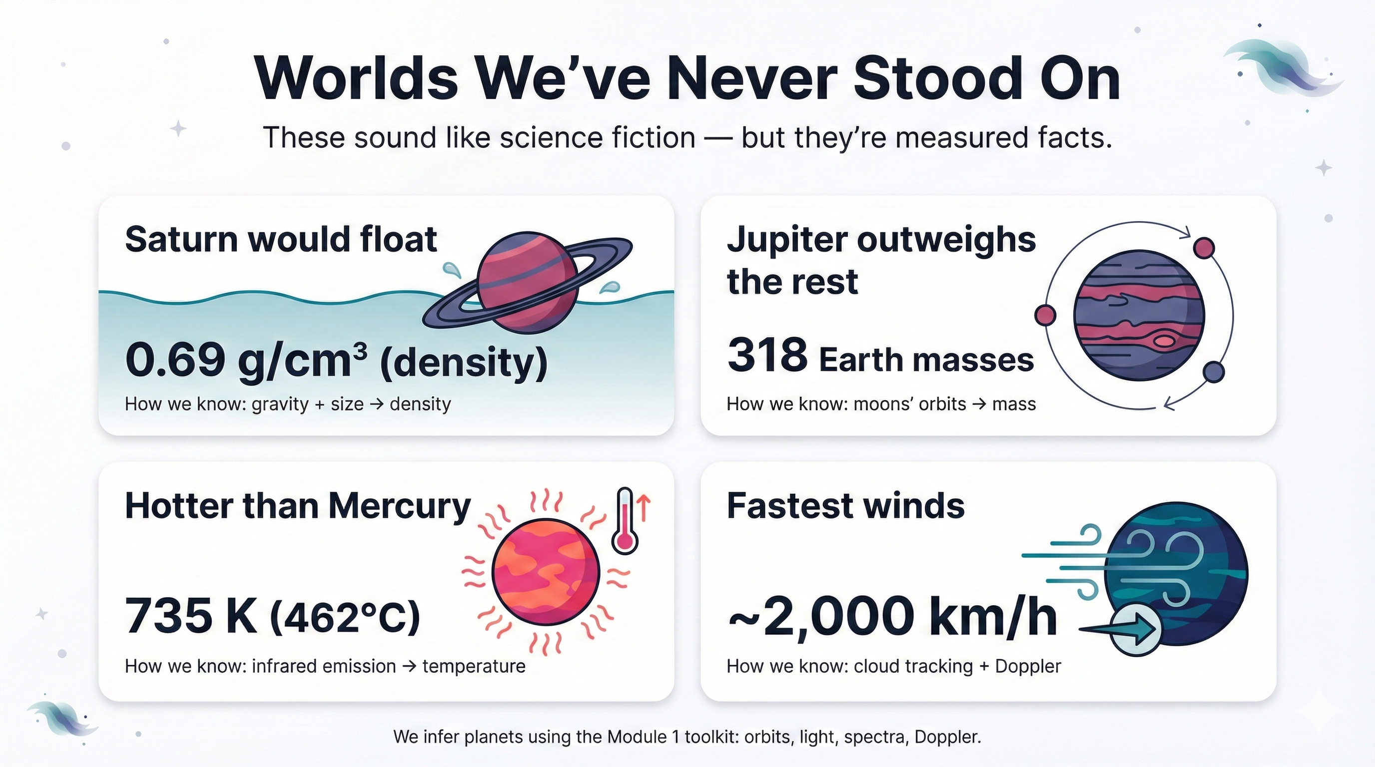
What to notice: we can infer basic planet properties (mass, density, temperature, winds) without visiting — by combining orbits, light, spectra, and Doppler. (Credit: (A. Rosen/Gemini — illustrative))
Saturn would float in water — its density is about 0.69 \(g/cm^{3},\) less than water’s 1.0 \(g/cm^{3}.\)
Jupiter outweighs all the other planets combined — about 318 Earth masses.
Venus is hotter than Mercury, even though it’s farther from the Sun — about \(460^{\circ}\)C at the surface, hot enough to melt lead.
Neptune has the fastest winds in the solar system — roughly 2,000 km/h, several times faster than the strongest hurricanes on Earth.
How do we know these are true? That’s what this lecture is about.
Over the past weeks, you’ve assembled a powerful toolkit: Kepler’s Laws describe orbits. Newton’s gravity reveals mass. Blackbody radiation encodes temperature. Spectral lines fingerprint composition. The Doppler effect measures motion.
Now we apply these tools to our own solar system — the best practice ground we have.
Take 2 minutes to answer these from memory (no peeking!):
- Kepler’s Third Law relates which two quantities?
- Doppler effect measures which component of velocity — radial or transverse?
- Wien’s Law lets you infer what property from a spectrum?
If you struggled, review the relevant lecture before continuing. This reading assumes you have these tools ready to apply.
- Period and semi-major axis (\(P^2 \propto a^3\))
- Radial (line-of-sight)
- Temperature from peak wavelength
| Tool | From Lecture | Solar System Application |
|---|---|---|
| Kepler’s Laws | L5 | Orbital distances, periods, predicting positions |
| Newton’s Gravity | L6 | Planetary and moon masses from orbits |
| EM Spectrum | L7 | Observing planets at IR, radio, UV |
| Blackbody/Wien | L8 | Surface and atmospheric temperatures |
| Spectroscopy | L9 | Atmospheric compositions |
| Doppler Effect | L10 | Rotation rates, wind speeds |
This week: We apply ALL of these to planets, climate, exoplanets, and the search for life.
Part 1: Solar System Architecture
The Grand Tour
Our solar system has a clear structure, organized by distance from the Sun. Let’s take a tour from the scorching inner regions to the frozen outer reaches.
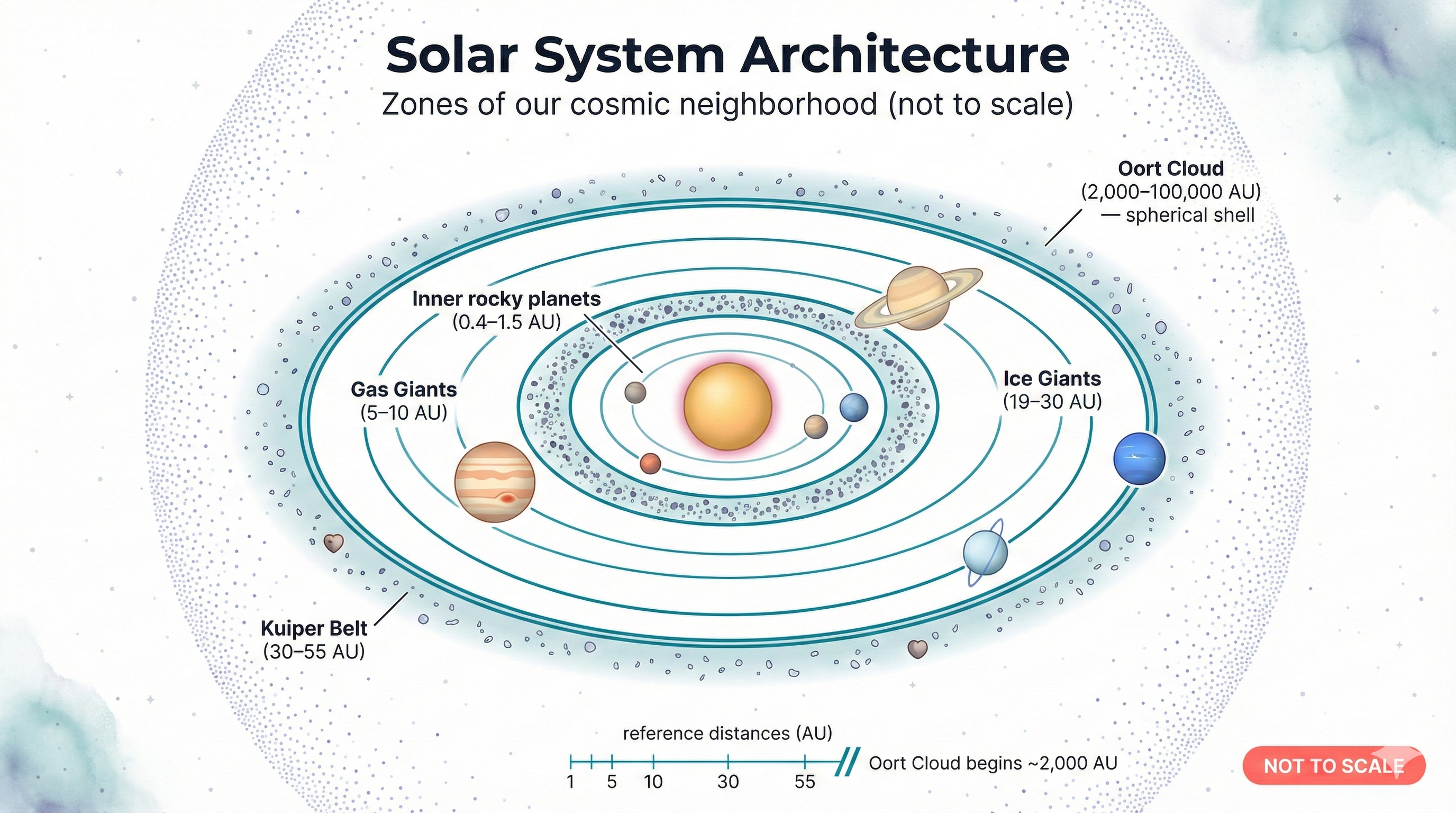
What to notice: the solar system is structured in zones (not to scale) — rocky planets inside, giant planets farther out, then icy small-body reservoirs (Kuiper Belt, Oort Cloud). (Credit: (A. Rosen/Gemini — illustrative))
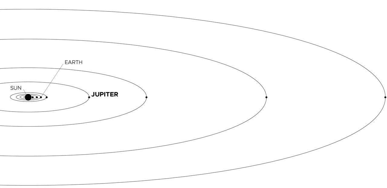
What to notice: Distances in the solar system are easiest to compare in AU — the inner planets are packed close together compared to the giant-planet region. (Credit: NASA)
The Zones
Think of the solar system as organized into distinct zones, each with characteristic objects:
The Inner Solar System (0.4–1.5 AU): This is the realm of the rocky planets — Mercury, Venus, Earth, and Mars. These worlds are small, dense, and have solid surfaces you could (in principle) stand on. They’re close enough to the Sun that temperatures would have been too high for ices to form when the solar system was young.
The Asteroid Belt (2–4 AU): Between Mars and Jupiter lies a ring of millions of rocky and metallic bodies — the asteroids. These are planetesimals that never accreted into a planet. Jupiter’s gravitational influence (especially through orbital resonances) kept collisions destructive rather than constructive, preventing a fifth rocky planet from forming.
The asteroid belt is not the wreckage of a planet that blew up. The total mass of the entire asteroid belt is only about 4% of the Moon’s mass — far too little to have ever been a planet. These are leftovers that never assembled in the first place, because Jupiter’s gravity stirred them up too violently. Also: the belt is mostly empty space. If you flew through it, you’d be unlikely to see two asteroids at the same time. Hollywood lied.
The Gas Giants (5–10 AU): Jupiter and Saturn dominate this region. These massive worlds are composed primarily of hydrogen and helium — the same elements that make up the Sun. They have no solid surface; if you tried to land, you’d sink through increasingly dense gas until pressure and temperature crushed you. Jupiter alone contains more mass than all other planets combined.
“Gas” is misleading. Despite the name, Jupiter isn’t a diffuse cloud. Deep inside, hydrogen is compressed to densities greater than lead and behaves as a metallic liquid. Jupiter’s core pressure is estimated at ~70 million atmospheres. “Gas giant” describes the composition (hydrogen, helium), not the state of matter throughout.
The Ice Giants (19–30 AU): Uranus and Neptune are often grouped with Jupiter and Saturn as “giant planets,” but they’re fundamentally different. They’re smaller, and instead of being hydrogen-dominated, they contain substantial amounts of water, ammonia, and methane ices. Their blue-green colors come from methane absorbing red light.
The Kuiper Belt (30–55 AU): Beyond Neptune lies a disk of icy bodies left over from the solar system’s formation. Pluto lives here, along with other dwarf planets like Makemake and Haumea. The Kuiper Belt is the source of many short-period comets. Scattered disk objects (like Eris) occupy even more eccentric and inclined orbits beyond the classical Kuiper Belt.
The Oort Cloud (~2,000–100,000 AU): At the outer edges of the Sun’s gravitational influence lies a vast spherical shell of icy bodies. The inner Oort Cloud (sometimes called the Hills Cloud) extends from roughly 2,000–20,000 AU; the outer cloud reaches from ~20,000 to perhaps 100,000 AU. Objects here are so loosely bound that passing stars and the Milky Way’s gravity can nudge them into the inner solar system as long-period comets.
Astronomical Unit (AU): The average Earth-Sun distance, ~150 million km. A convenient unit for solar system distances.
The Key Pattern
Notice something striking: rocky planets are close to the Sun; gas giants are far away. This isn’t random — it’s a direct consequence of how the solar system formed. We’ll explain why in Part 3.
| Zone | Distance | Objects | Key Properties |
|---|---|---|---|
| Rocky planets | 0.4–1.5 AU | Mercury, Venus, Earth, Mars | Small, dense, solid surfaces |
| Asteroid belt | 2–4 AU | Millions of rocky/metallic bodies | Planetesimals that never formed a planet |
| Gas giants | 5–10 AU | Jupiter, Saturn | Massive, H/He dominated, no solid surface |
| Ice giants | 19–30 AU | Uranus, Neptune | Smaller, more ices (water, ammonia, methane) |
| Kuiper Belt | 30–55 AU | Pluto, dwarf planets, icy bodies | Source of short-period comets |
| Oort Cloud | ~2,000–100,000 AU | Long-period comets | Spherical halo, barely bound to Sun |
The inner solar system (0.4–1.5 AU) contains rocky planets; the outer solar system (5–30 AU) contains gas and ice giants. If you could magically move Jupiter to Earth’s orbit (1 AU), would it remain a gas giant?
- Yes — Jupiter would keep its hydrogen/helium atmosphere regardless of location
- No — the Sun’s heat would immediately boil away all the gas
- It depends — Jupiter is massive enough to hold its gas now, but it could not have formed as a gas giant at 1 AU
- No — rocky planets can only exist close to the Sun
C) It depends — Jupiter is massive enough to hold its gas now, but it could not have formed as a gas giant at 1 AU.
Jupiter’s gravity is strong enough to retain its atmosphere today — even at 1 AU. But during formation, the inner solar system was too hot for ices to condense. Without ices, rocky cores there grew too slowly to capture gas before the solar nebula dispersed (~3–10 million years). The key insight: where a planet forms determines what it becomes. The frost line (Part 3) is a formation boundary, not a survival boundary. This is why “hot Jupiters” — gas giants orbiting very close to their host stars — are thought to have migrated inward after forming farther out.
Rocky vs. Giant Planets: Two Families
The planets divide neatly into two families with dramatically different properties:
| Property | Rocky (Terrestrial) | Giants |
|---|---|---|
| Size | Small (0.4–1 \(R_\oplus\)) | Large (~4–11 \(R_\oplus\)) |
| Mass | Low (0.06–1 \(M_\oplus\)) | High (~15–318 \(M_\oplus\)) |
| Density | High (3.9–5.5 \(g/cm^{3})\) | Low (0.69–1.6 \(g/cm^{3})\) |
| Composition | Rock, metal | H, He, ices |
| Surface | Solid | None (gas/liquid) |
| Moons | Few (0–2) | Many (dozens) |
| Rings | None | Yes |
The density difference is particularly striking. Earth’s density is 5.5 \(g/cm^{3}\) — about five times denser than water. Saturn’s density is just 0.69 \(g/cm^{3}\) — less than water. If you could find an ocean big enough, Saturn would float!
Students learn patterns faster through paired comparisons. As you read, think about these contrasts:
Mercury vs. Venus: Both inner planets, but Mercury has no atmosphere (extreme temperature swings: \(430^{\circ}\)C day, -\(180^{\circ}\)C night) while Venus has a thick atmosphere (constant \(460^{\circ}\)C everywhere). Same region, different fates.
Venus vs. Earth: Nearly the same size, but Venus receives \(~2\times\) Earth’s sunlight (0.72 AU vs. 1.0 AU) and is \(450^{\circ}\)C hotter. Why so extreme? (Answer in L12: runaway greenhouse effect.)
Jupiter vs. Saturn: Both gas giants with similar composition, but Saturn’s density (0.69 \(g/cm^{3})\) is lower than water’s. Why? Saturn is less massive, so less compressed.
These comparisons reveal what physics is doing.
It’s tempting to think “closer to the Sun = hotter planet.” Mercury is closest, so it must be the hottest, right? Wrong. Venus (at 0.72 AU) is \(460^{\circ}\)C — hotter than Mercury’s dayside (\(430^{\circ}\)C) — even though Venus is almost twice as far from the Sun. The reason: Venus has a massive \(\mathrm{CO_{2}}\) atmosphere that traps heat (greenhouse effect). Distance sets the baseline, but atmosphere determines the outcome. We’ll quantify this in L12.
Saturn has a density of 0.69 \(g/cm^{3}\) — less than water. What does this tell you about its composition?
- It must be made of rock and metal
- It must be made primarily of lightweight gases (hydrogen, helium)
- It has no atmosphere
- It’s the same composition as Earth
B) It must be made primarily of lightweight gases (hydrogen, helium). Rocky planets have densities of 4-5 \(g/cm^{3}.\) Saturn’s low density tells us it’s dominated by hydrogen and helium, the lightest elements. If you could find a big enough ocean, Saturn would float!
A Quick Photo Tour (One World at a Time)
Pictures help your intuition. As you read the rest of this lecture, keep asking the same question: What does this world look like, and what physics makes it that way?
Rocky planets: solid surfaces, big contrasts
As you tour the inner solar system, notice how atmosphere thickness determines surface conditions — even for planets in the same region.
Mercury is the endmember for “no atmosphere.” Its surface is a cratered record of early impacts, and its temperature swings are extreme because there’s essentially no air to move heat around.
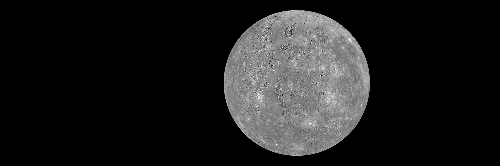
What to notice: Mercury’s surface is heavily cratered and airless — a record of early impacts with little erosion. (Credit: NASA)
Venus is the opposite: in visible light we don’t see a rocky surface at all, just a bright, global cloud deck. The climate physics lives in the atmosphere.
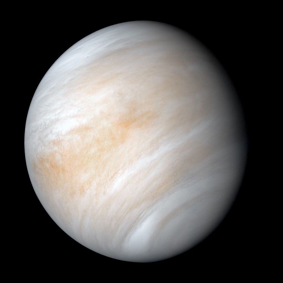
What to notice: Venus is completely cloud-covered in visible light — we do not see the surface directly without using other wavelengths or radar. (Credit: NASA)
Mercury vs. Venus: Both are inner planets, yet Mercury swings 610\(^\circ\)C between day and night while Venus holds steady at 460\(^\circ\)C everywhere. The key difference? Atmosphere. We’ll explore this contrast in L12.
Earth is our control case — oceans, clouds, and an atmosphere thick enough to matter.
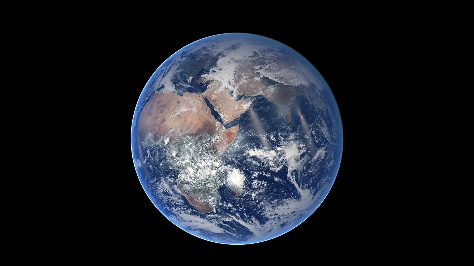
What to notice: Earth’s oceans and atmosphere matter — they shape temperature, weather, and habitability. (Credit: NASA)
Mars is a reminder that “rocky” doesn’t mean “Earth-like.” A thin atmosphere changes the climate story.
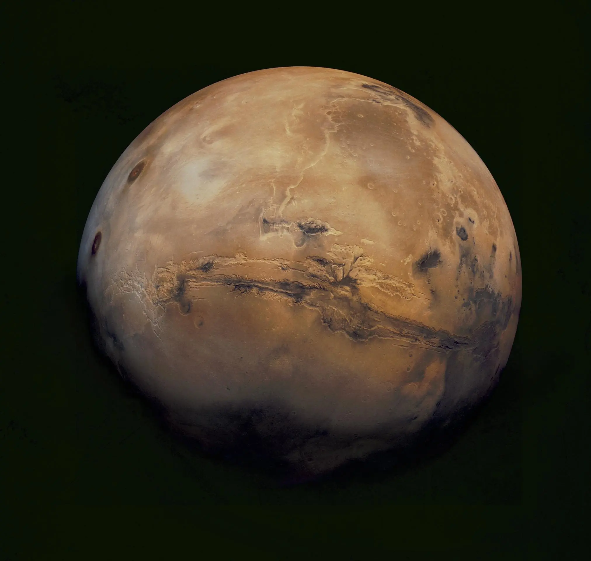
What to notice: Mars is a cold, rocky world with a thin atmosphere — a contrast case for climate and habitability. (Credit: NASA)
Mars also has two tiny, irregular moons — more like captured asteroids than scaled-down versions of our Moon.
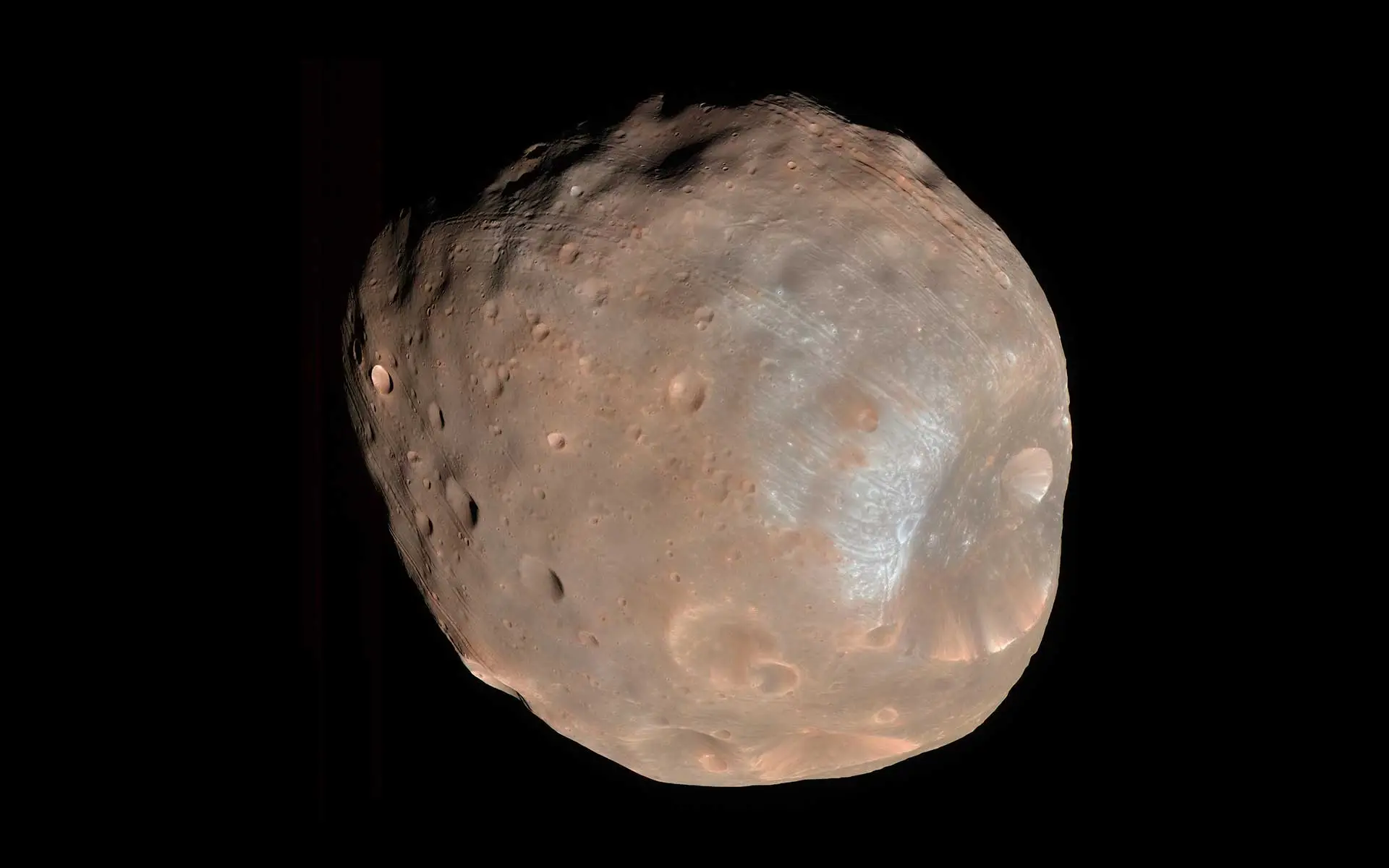
What to notice: Small moons can be irregular and heavily cratered — they look more like asteroids than planets. (Credit: NASA)
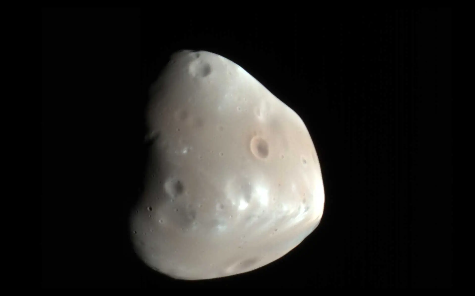
What to notice: Deimos is tiny and irregular — evidence that not all moons form the same way.
You’ve now seen the four rocky planets. Before moving on, notice the pattern:
- Mercury: No atmosphere \(\rightarrow\) extreme temperature swings, cratered surface
- Venus: Thick atmosphere \(\rightarrow\) uniform extreme heat, cloud-covered
- Earth: Moderate atmosphere \(\rightarrow\) habitable conditions, oceans
- Mars: Thin atmosphere \(\rightarrow\) cold, dry, some evidence of past water
The key variable is atmosphere. Same region of space, same rocky composition, but wildly different outcomes depending on atmospheric thickness. Keep this pattern in mind as we tour the outer solar system.
The asteroid belt: leftovers and building blocks
The asteroid belt is made of leftovers, not “mini-planets.” But it still contains large bodies — including the dwarf planet Ceres.
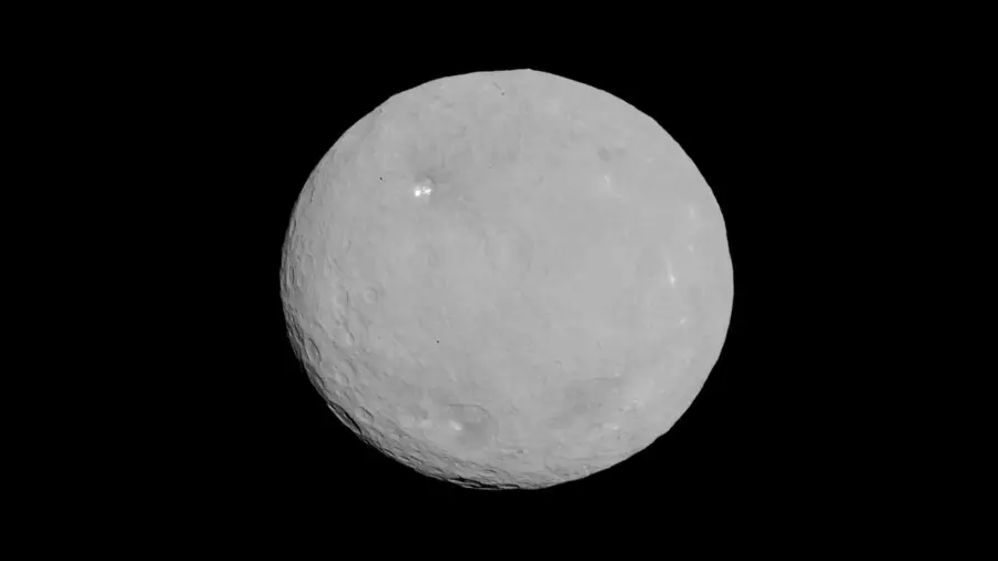
What to notice: The asteroid belt contains large bodies too — Ceres is a dwarf planet with its own geology. (Credit: NASA)
Giant planets: atmospheres without a surface
Jupiter and Saturn are dominated by atmosphere: bands, storms, and deep fluid layers. The familiar “surface” is actually cloud tops.
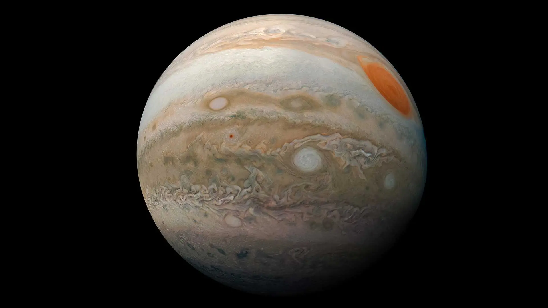
What to notice: Jupiter is a gas giant with banded cloud layers — atmosphere, not a solid surface, dominates what we see. (Credit: NASA)
Saturn adds the most obvious disk in the solar system: its rings.
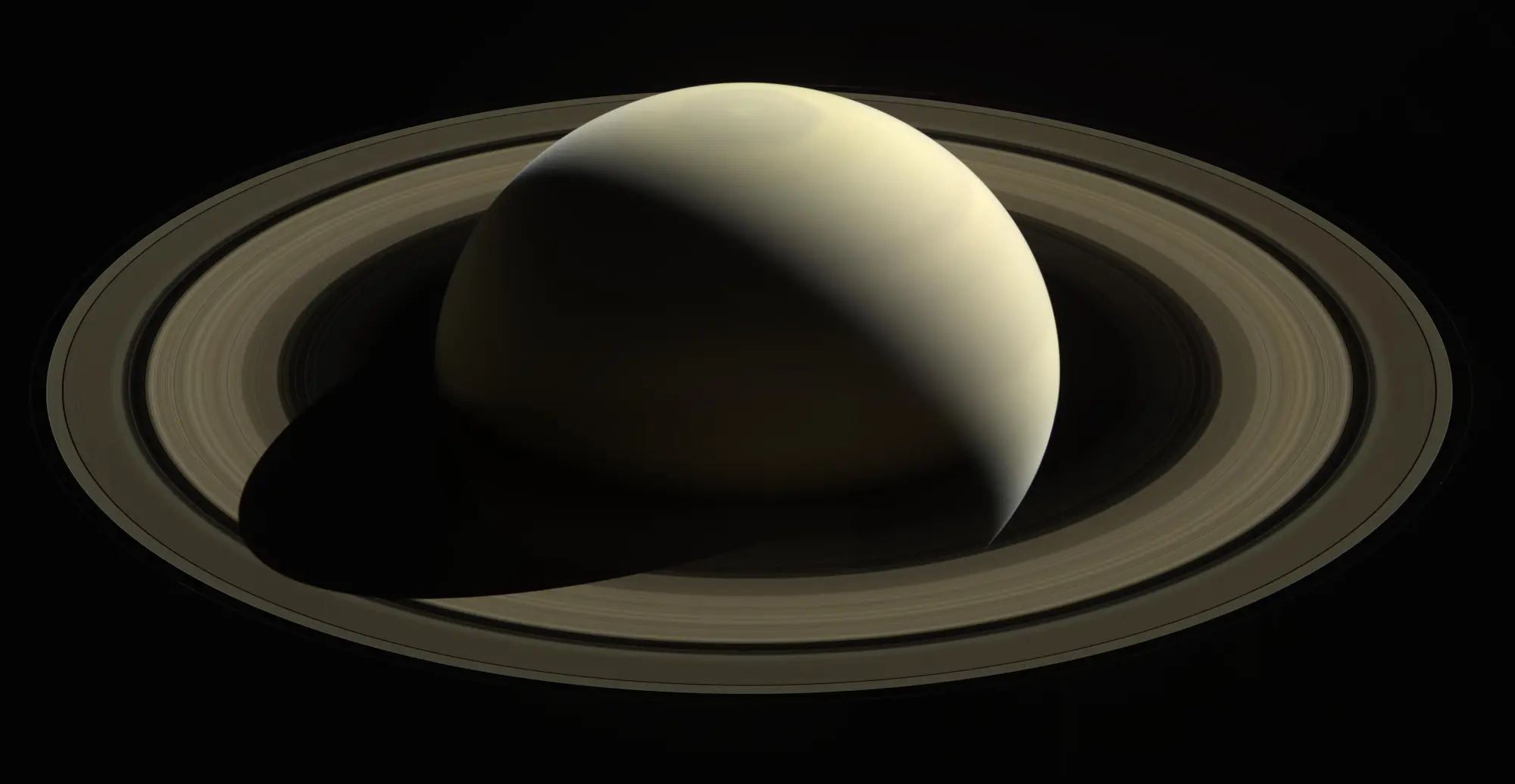
What to notice: Saturn’s rings make its structure obvious: a planet plus a disk of countless small particles. (Credit: NASA)
Jupiter vs. Saturn: Both are gas giants with similar composition, but Saturn’s density (0.69 g/cm\(^3\)) is less than water while Jupiter’s (1.33 g/cm\(^3\)) is not. Why? Saturn is less massive, so less gravitationally compressed.
And moons can be worlds too — Titan has a thick atmosphere that hides its surface in visible light.
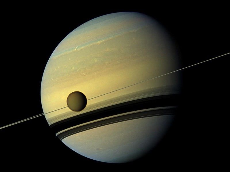
What to notice: Titan is a moon with a thick atmosphere — moons can have their own ‘planet-like’ complexity. (Credit: NASA)
Jupiter’s average density is 1.33 \(g/cm^{3}\) — slightly above water. Saturn’s is 0.69 \(g/cm^{3}\) — below water. Both are “gas giants” made mostly of hydrogen and helium. Why is Jupiter denser than Saturn despite having similar composition?
- Jupiter has more rock and metal in its core
- Jupiter’s greater mass compresses its gas to higher density
- Saturn’s rings remove mass, lowering its density
- Jupiter is closer to the Sun, so its gas is hotter and denser
B) Jupiter’s greater mass compresses its gas to higher density.
Jupiter is \(\sim 3\times\) more massive than Saturn, and that extra mass creates enormous pressure in the interior. At Jupiter’s core, pressures reach \(\sim 70\) million atmospheres, compressing hydrogen into a metallic liquid denser than lead. More mass \(\rightarrow\) more gravity \(\rightarrow\) more compression \(\rightarrow\) higher average density. This is a general pattern: among gas giants, the most massive ones are actually the densest because gravity squeezes them. (Option A contributes a small amount — Jupiter does have a larger core — but the dominant effect is gravitational compression of the envelope.)
Ice giants and beyond: cold, distant, and still active
Uranus and Neptune are colder and smaller than Jupiter and Saturn, with different compositions and atmospheric chemistry.
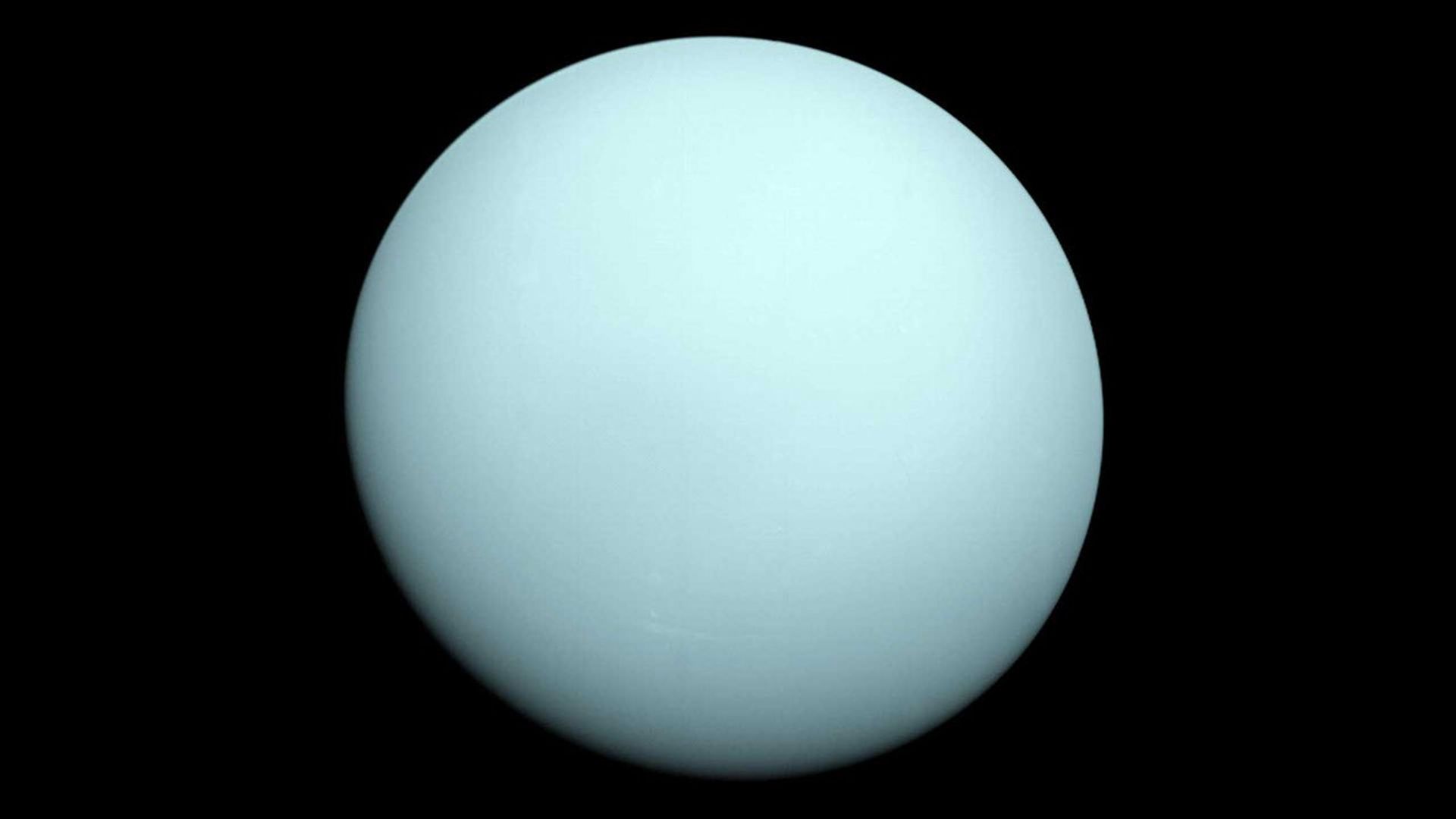
What to notice: The ice giants are distant and cold — their atmospheres and compositions differ from Jupiter and Saturn. (Credit: NASA)
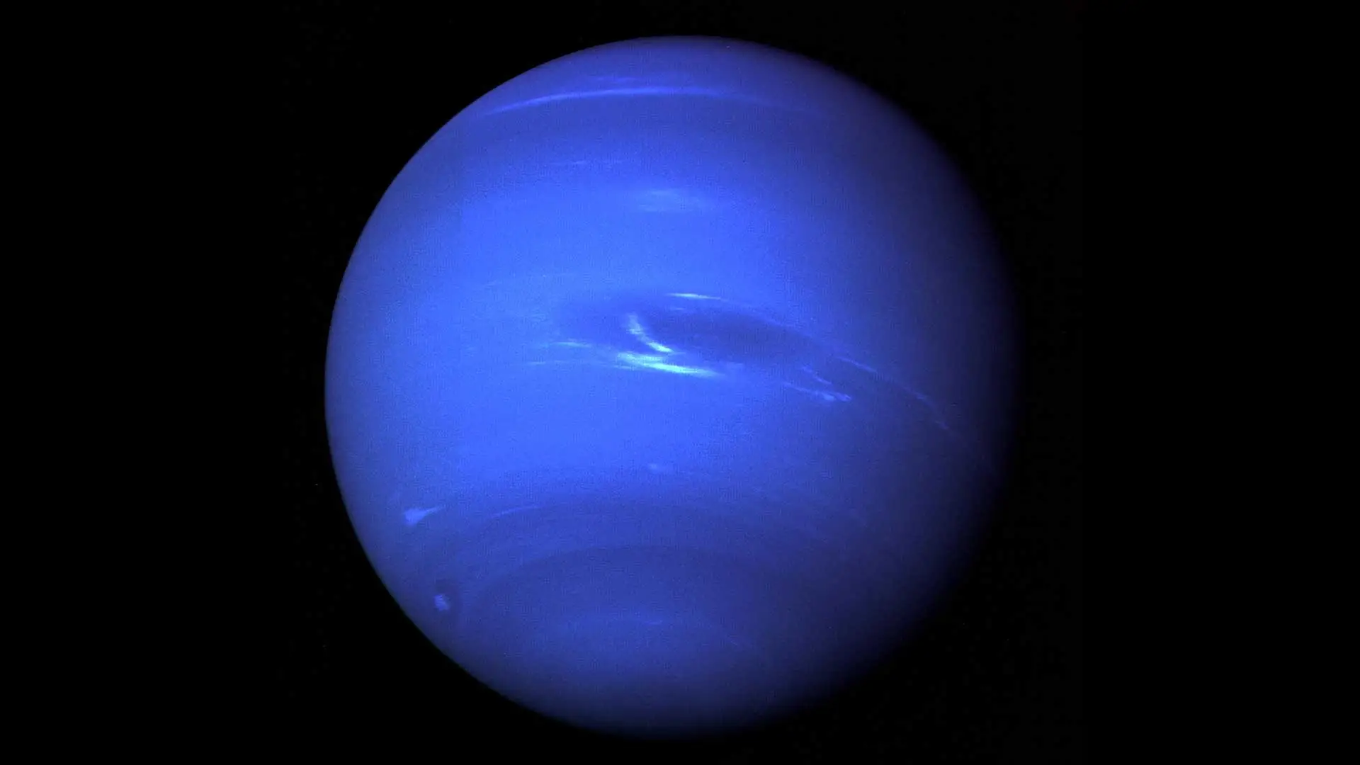
What to notice: Neptune’s deep blue color and storms emphasize that ice giant atmospheres can be active. (Credit: NASA)
Quick question: Uranus and Neptune appear blue-green. Using what you learned in L9 (spectroscopy), what molecule in their atmospheres might cause this color? Think about it before reading the answer in the composition section below.
Pluto is a signpost: the outer solar system contains many icy worlds and dwarf planets beyond the eight planets.
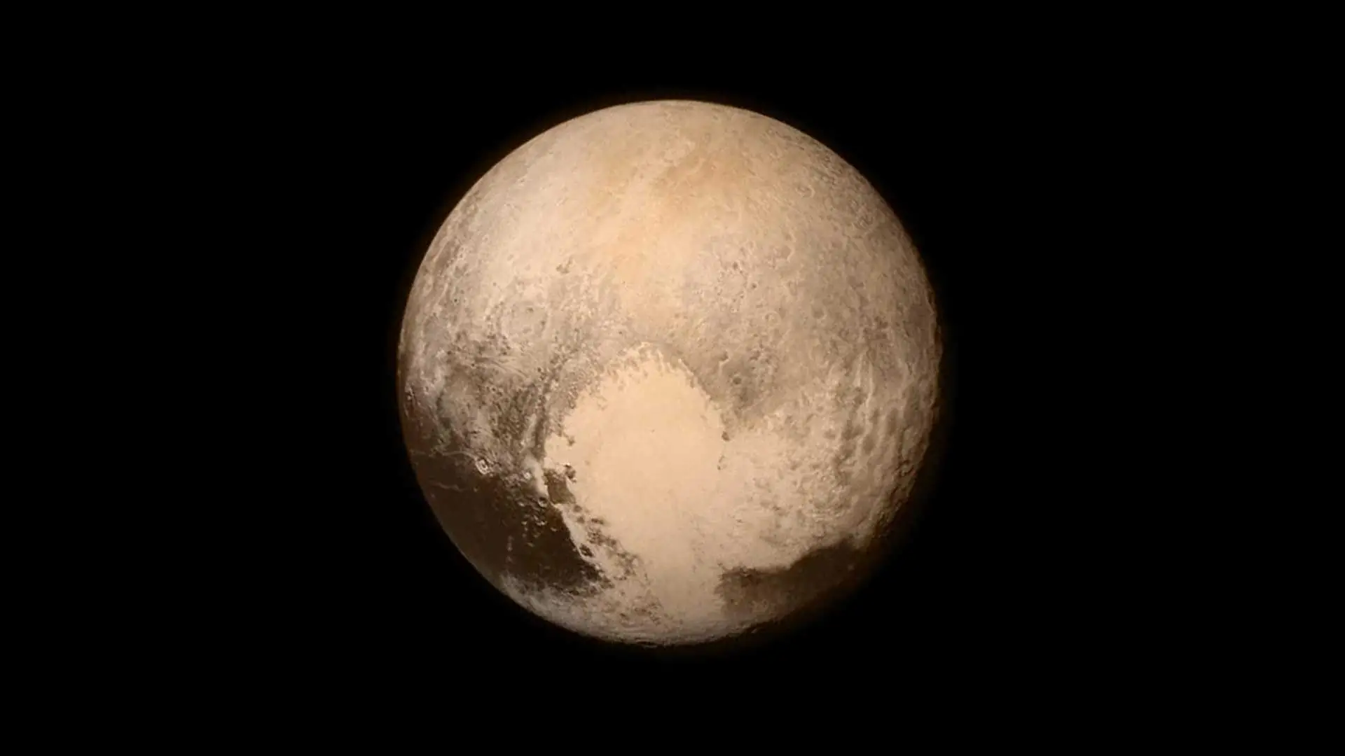
What to notice: Pluto lives in the Kuiper Belt — the outer solar system includes dwarf planets and icy worlds, not just the eight planets. (Credit: NASA)
Almost every close-up photo in this section exists because of two spacecraft: Voyager 1 and Voyager 2, launched in 1977. They took advantage of a rare planetary alignment that occurs roughly once every 175 years, allowing gravity assists to slingshot from planet to planet.
Voyager 2 remains the only spacecraft ever to visit Uranus and Neptune. Both Voyagers have now crossed into interstellar space — beyond the Sun’s influence — and are still sending data back to Earth after nearly 50 years. The farthest human-made objects in the universe, carrying golden records with sounds and images of Earth.
Part 2: Applying Our Toolkit
How Do We Know What We Know?
We’ve never brought back samples from Jupiter. We’ve never landed on Neptune. Yet we know their masses, compositions, temperatures, and rotation rates. How?
Everything comes from the physics of Module 1.
This is the power of remote sensing. Light carries information across billions of kilometers, and our toolkit lets us decode it.
| What We Measure | The Tool | The Physics |
|---|---|---|
| Distance from Earth | Radar ranging | Round-trip light travel time |
| Distance from Sun (a) | Kepler III (once P known) | \(P^2 \propto a^3\) |
| Orbital period | Observation over time | Track position against stars |
| Mass (with moons) | Moon orbits + Newton | \(M = \frac{4\pi^2 a^3}{GP^2}\) |
| Mass (no moons) | Spacecraft tracking | Gravity bends spacecraft path |
| Temperature | IR spectrum + Wien | Peak wavelength \(\rightarrow\) temperature |
| Composition | Spectral lines | Absorption/emission fingerprints |
| Rotation rate | Repeated imaging + Doppler | Track patterns; measure broadening |
| Wind speeds | Doppler + cloud tracking | Line-of-sight speeds; pattern motion |
Worked Example: Jupiter’s Mass from Io’s Orbit
Let’s apply Newton’s form of Kepler’s Third Law to measure Jupiter’s mass.
Problem: Jupiter’s moon Io orbits at a = 422,000 km with period P = 1.77 days. Find Jupiter’s mass.
Solution:
Step 1: Convert units to SI
- \(a = 422{,}000 \text{ km} = 4.22 \times 10^{8} \text{ m}\)
- \(P = 1.77 \text{ days} \times 86{,}400 \text{ s/day} = 1.53 \times 10^{5} \text{ s}\)
Step 2: Apply Newton’s version of Kepler III
\[ M = \frac{4\pi^2 a^3}{GP^2} \]
where \(G = 6.674 \times 10^{-11} \text{ m}^3 \text{ kg}^{-1} \text{ s}^{-2}\).
Step 3: Compute numerator and denominator separately (with units!)
Numerator:
\[ 4\pi^2 \, a^3 = 4\pi^2 \times (4.22 \times 10^{8} \text{ m})^3 = 39.48 \times 7.51 \times 10^{25} \text{ m}^3 = 2.96 \times 10^{27} \text{ m}^3 \]
Denominator:
\[ G \, P^2 = (6.674 \times 10^{-11} \text{ m}^3 \text{ kg}^{-1} \text{ s}^{-2}) \times (1.53 \times 10^{5} \text{ s})^2 \]
\[ = 6.674 \times 10^{-11} \text{ m}^3 \text{ kg}^{-1} \text{ s}^{-2} \times 2.34 \times 10^{10} \text{ s}^2 = 1.56 \text{ m}^3 \text{ kg}^{-1} \]
Step 4: Divide — units cancel to kg
\[ M = \frac{2.96 \times 10^{27} \text{ m}^3}{1.56 \text{ m}^3 \text{ kg}^{-1}} = 1.9 \times 10^{27} \text{ kg} \]
The \(\text{m}^3\) cancels, and dividing by \(\text{kg}^{-1}\) flips to \(\text{kg}\). We get kilograms, as expected for a mass.
This is 318 Earth masses — determined entirely by watching Io orbit! We never touched Jupiter. We just measured Io’s orbit and applied Newton’s gravity.
Observable: Io orbits Jupiter at 422,000 km with period 1.77 days. (Position + Timing)
Model: Newton’s form of Kepler III: \(M = 4\pi^2 a^3 /(GP^2)\)
Inference: Jupiter’s mass is \(1.9 \times 10^{27}\) kg = 318 Earth masses.
Same pattern as always: measurement \(\rightarrow\) physics \(\rightarrow\) knowledge.
If a planet has a moon orbiting at twice the distance but with the same orbital period, what can you conclude about the planet’s mass compared to another planet with the original moon orbit?
- The same mass
- \(2\times\) the mass
- \(4\times\) the mass
- \(8\times\) the mass
D) \(8\times\) the mass. From \(M = 4\pi^2 a^3 /(GP^2)\), if \(a\) doubles and \(P\) stays the same, \(M\) must increase by \(2^3 = 8\) times. Larger orbits at the same period require stronger gravity \(\rightarrow\) more mass.
Which tool would you use to measure Jupiter’s mass if it had NO moons?
- Wien’s Law
- Spectroscopy
- Track a spacecraft’s path as it flies by
- Doppler effect on Jupiter’s light
C) Track a spacecraft’s path as it flies by. Without moons, we can’t use Newton’s form of Kepler III. But a spacecraft passing Jupiter gets deflected by gravity — by measuring how much the path bends, we can calculate Jupiter’s mass. This is how we measure masses of moonless asteroids and comets.
Temperature from Wien’s Law
Planets Glow in the Infrared
Every planet emits thermal radiation. Using Wien’s Law from L8:
\[ \lambda_{\text{peak}} = \frac{2.9 \times 10^6 \text{ nm\cdot K}}{T} \]
We can measure a planet’s peak emission wavelength and calculate its temperature. For most planets, this peak is in the infrared — invisible to our eyes but detectable by IR telescopes.
Observable: A planet’s thermal emission peaks at a specific infrared wavelength. (Wavelength)
Model: Wien’s Law: \(\lambda_{\text{peak}} = 2.9 \times 10^6 \text{ nm\cdot K} /T\)
Inference: The planet’s temperature. Neptune peaks at ~50,000 nm \(\rightarrow\) \(T \approx 58\) K. Same physics as reading a star’s temperature from its color — just shifted to infrared.
Equilibrium Temperature: A Baseline Prediction
Equilibrium temperature is what a planet’s temperature would be if:
- It absorbed sunlight and re-radiated as a blackbody
- It had no atmosphere (no greenhouse effect)
- Temperature was averaged over the whole surface
The idea comes straight from Stefan-Boltzmann (L8): the Sun pours energy onto the planet, and the planet radiates energy back to space. When energy in = energy out, you get a steady temperature — the equilibrium value. It’s a baseline prediction. When the observed temperature differs from equilibrium, something interesting is happening.
Equilibrium temperature is a prediction — what physics says “should” happen with just sunlight in, thermal radiation out.
Observed temperature is what we measure.
When they differ, something interesting is happening:
- Venus: Observed >> Equilibrium \(\rightarrow\) massive greenhouse effect
- Jupiter: Observed > Equilibrium \(\rightarrow\) internal heat source
- Mercury: Observed \(\approx\) Equilibrium (on average) \(\rightarrow\) no atmosphere
Always compare the two to diagnose what’s going on!
Planetary Temperature Comparison
How to read this table: Compare the equilibrium column (what physics predicts with no atmosphere) to the observed column (what we actually measure). When they differ, the gap tells you something — a greenhouse effect, an internal heat source, or a missing atmosphere. Look for the biggest mismatches.
| Planet | Distance (AU) | T_equilibrium (K) | T_observed (K) | Notes |
|---|---|---|---|---|
| Mercury | 0.39 | ~440 | ~90–700 | No atmosphere \(\rightarrow\) extreme day/night swing |
| Venus | 0.72 | ~230 | 735 | Runaway greenhouse! |
| Earth | 1.0 | ~255 | 288 | Moderate greenhouse (+33 K) |
| Mars | 1.52 | ~210 | 218 | Thin atmosphere (+8 K) |
| Jupiter | 5.2 | ~110 | ~165 | Internal heat source adds ~55 K |
Mercury never actually reaches ~440 K uniformly — with no atmosphere to redistribute heat, the dayside soars to ~700 K while the nightside plunges to ~90 K. The equilibrium value is a useful theoretical baseline, not a real surface temperature.
Mercury’s extremes illustrate what happens without an atmosphere: daytime reaches 700 K (\(430^{\circ}\)C), but nighttime plunges to 90 K (-\(180^{\circ}\)C). That \(610^{\circ}\)C swing would be impossible with an atmosphere to redistribute heat.
Technically, Mercury has an exosphere — an extremely thin envelope of atoms (sodium, potassium, oxygen, hydrogen) that are constantly escaping to space and being replenished by solar wind bombardment, micrometeorite impacts, and outgassing from the surface.
The exosphere is so thin (surface pressure \(< \sim 10^{-12}\,\mathrm{bar}\), compared to Earth’s 1 bar) that atoms rarely collide with each other. It provides essentially no insulation, no heat redistribution, no greenhouse effect — which is why Mercury’s temperature swings are so extreme.
For our purposes: Mercury effectively has “no atmosphere” in the thermodynamic sense that matters for climate.
Venus stands out: its actual temperature is 500 K hotter than equilibrium! This is the greenhouse effect at its most extreme — and we’ll explore it in L12.
Venus is nearly Earth’s twin in size and mass. Scientists believe it may have had Earth-like conditions early in its history — possibly even liquid water oceans. So what went wrong?
In L12, we’ll trace Venus’s transformation from potentially habitable world to 735 K hellscape. The culprit: a runaway greenhouse effect triggered by Venus being slightly too close to the Sun. It’s a story with implications for understanding climate here on Earth.
Jupiter is warmer than equilibrium because it has an internal heat source — leftover heat from its formation, still slowly radiating away after 4.6 billion years.
Mercury and Venus are both “hot” planets. Which tool would help you distinguish “hot because close to Sun” from “hot because greenhouse effect”?
- Compare observed temperature to equilibrium temperature
- Measure the planet’s mass
- Count the planet’s moons
- Measure the planet’s orbital period
A) Compare observed temperature to equilibrium temperature. Mercury’s temperature roughly matches what you’d expect from its distance (equilibrium). Venus is 500 K hotter than equilibrium — that huge gap reveals the greenhouse effect is doing something extreme. This is exactly how we diagnosed Venus’s climate.
Compositions from Spectroscopy
Atmospheric Fingerprints
By observing planets at different wavelengths and looking for spectral lines (L9), we determine atmospheric compositions. Each molecule absorbs at specific wavelengths — its spectral fingerprint.
- Venus: \(\mathrm{CO_{2}}\) (96%), \(\mathrm{N_{2}}\) (3.5%), sulfuric acid clouds
- Earth: \(\mathrm{N_{2}}\) (78%), \(\mathrm{O_{2}}\) (21%), trace \(CO_{2},\) \(\mathrm{H_{2}O}\)
- Mars: \(\mathrm{CO_{2}}\) (95%), \(\mathrm{N_{2}}\) (2.7%), thin atmosphere
- Jupiter: \(\mathrm{H_{2}}\) (~90%), He (~10%), traces of \(CH_{4},\) \(NH_{3},\) \(\mathrm{H_{2}O}\)
The same spectroscopy that identifies elements in stars identifies molecules in planetary atmospheres! The physics is identical — just applied to different objects.
Observable: Absorption lines at specific wavelengths in sunlight reflected by a planet. (Wavelength)
Model: Each molecule absorbs at unique wavelengths — its spectral fingerprint (L9). CO\(_2\) absorbs at 4.3 \(\mu\)m and 15 \(\mu\)m; CH\(_4\) at 3.3 \(\mu\)m; H\(_2\)O across many IR bands.
Inference: Venus’s atmosphere is 96% CO\(_2\), Jupiter is 90% H\(_2\), Neptune contains CH\(_4\) (explaining its blue color). Same toolkit as stellar spectroscopy — different targets.
Here’s the key for L12: we can do this for planets orbiting other stars. When an exoplanet transits (passes in front of) its host star, starlight filters through the planet’s atmosphere on its way to us. Each atmospheric molecule imprints its absorption fingerprint on that light — exactly the same spectroscopy we just used on Venus, Earth, and Jupiter. Same physics, different distance.
Color as a Clue
Sometimes a planet’s color hints at its composition. Neptune and Uranus appear blue-green because methane \((CH_{4})\) in their atmospheres absorbs red light, leaving the blue to be reflected back to us.
Mars appears red for a different reason — not atmospheric absorption, but iron oxide (rust!) on its surface.
In everyday life, blue often means cold (ice, cold water). But in astronomy, a planet’s color has nothing to do with its temperature in any simple way. Neptune is blue because methane absorbs red light — it’s a chemistry effect, not a temperature effect. Meanwhile, a blue star (like Rigel) is blue because it’s extremely hot — the opposite of the everyday association. Always ask: what physical process produces this color?
Mars appears red to our eyes. Neptune appears blue. Using concepts from L7-L9, which planet likely has methane \((CH_{4})\) in its atmosphere?
- Mars — red color means methane
- Neptune — methane absorbs red light, leaving blue
- Both have methane
- Neither has methane
B) Neptune — methane absorbs red light, leaving blue. Spectroscopy confirms that Neptune (and Uranus) have methane in their atmospheres. Methane absorbs red wavelengths, so the reflected sunlight appears blue. Mars is red because of iron oxide (rust) on its surface, not atmospheric absorption.
An alien astronomer observes Earth from 100 light-years away. They detect O\(_2\) and N\(_2\) in our atmosphere. Which Module 1 tool are they using?
- Kepler’s Third Law
- Wien’s Law
- Spectroscopy
- The Doppler effect
C) Spectroscopy. Each molecule absorbs at unique wavelengths — its spectral fingerprint (L9). The alien astronomer sees sunlight that has passed through Earth’s atmosphere, with absorption lines from O\(_2\) and N\(_2\) imprinted on the spectrum. This is exactly how we study exoplanet atmospheres (coming in L12)!
Part 3: Solar System Formation
The solar system’s layout is fossil evidence. Rocky worlds huddle inside. Gas giants patrol the outer system. A belt of rubble sits where a fifth rocky planet might have formed. Icy debris extends to the edge of the Sun’s gravitational influence.
This isn’t random. It’s the preserved record of what happened 4.6 billion years ago. If we can read the pattern, we can reconstruct the story.
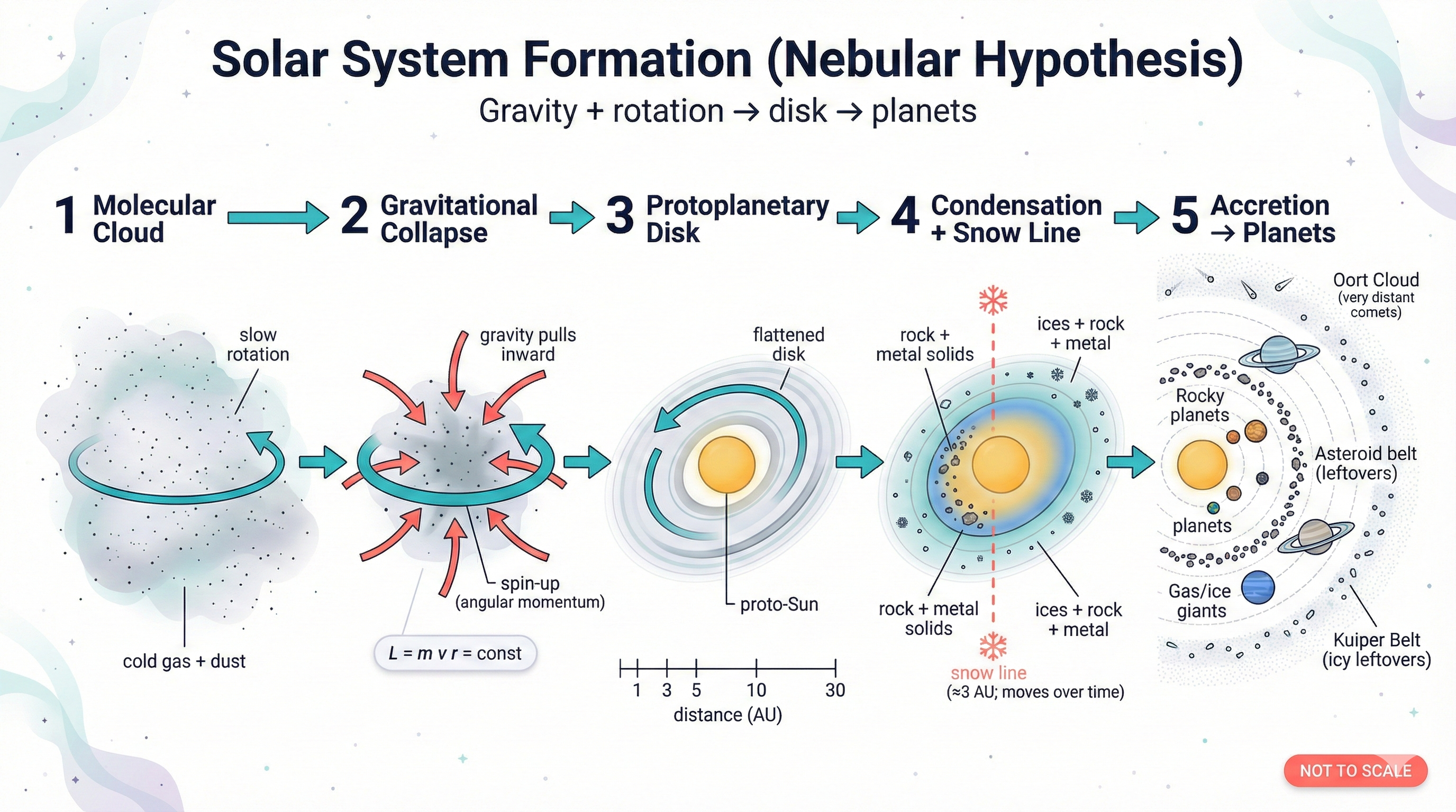
The Nebular Hypothesis
How did the solar system form? The leading model — the nebular hypothesis — explains why the solar system looks the way it does.
The solar system formed ~4.6 billion years ago from a collapsing cloud of gas and dust called the solar nebula. Here’s the cause \(\rightarrow\) effect chain:
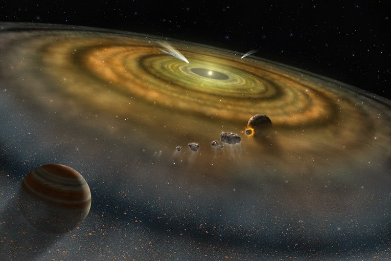
What to notice: The nebular hypothesis starts with a rotating disk of gas and dust. Collisions and gravity flatten the system into a plane, which is why most planets end up orbiting in nearly the same plane and direction.
1. Gravity \(\rightarrow\) Collapse
A region of a molecular cloud becomes dense enough to collapse under its own gravity.
2. Collapse \(\rightarrow\) Spin-up (Angular momentum conservation)
As the cloud shrinks, it spins faster — just like a figure skater pulling in their arms.
3. Spin-up + Collisions \(\rightarrow\) Disk
Rotation + collisions damp vertical motions, so material settles into a thin disk while continuing to orbit the center.
4. Temperature gradient \(\rightarrow\) Condensation sequence
Inner disk is hot (only rock/metal condenses); outer disk is cold (ices also condense).
5. Core growth outside snow line \(\rightarrow\) Gas capture
More solid material \(\rightarrow\) bigger cores \(\rightarrow\) gravitational capture of H/He \(\rightarrow\) gas giants.
But there’s a deadline. The hydrogen and helium gas in the nebula doesn’t last forever — radiation and winds from the young Sun blow it away within roughly 3–10 million years. Cores that grow massive enough before the gas disappears capture thick atmospheres and become gas giants. Cores that are still too small when the gas dissipates become ice giants (like Uranus and Neptune) or stay rocky. It’s a race against time.
Memorize this ladder. You can reconstruct the whole story from these five steps.
Why a disk, not a sphere? Collisions between particles are inelastic — they convert kinetic energy into heat. Random motions (up, down, sideways) lose energy and die out. But angular momentum is conserved, so the rotation can’t stop. The lowest-energy state consistent with conservation of angular momentum is a thin disk.
In plain English: A cloud of gas collapsed, spun into a pizza-dough disk, the inner disk was hot (rock only), the outer disk was cold (rock + ice), and the icy outer cores grew big enough to grab gas. That’s the whole story.
What to notice: formation as a causal chain — collapse spins up a rotating disk, temperature sets a condensation sequence, and the snow line separates rocky from ice-rich building blocks. (Credit: (A. Rosen/Gemini — illustrative))
Angular Momentum: The L5-L6 Connection
Remember the figure skater from L5? Arms out = slow spin; arms in = fast spin.
The same physics explains why the solar nebula spun up as it collapsed:
\[ L = mvr = \text{constant} \quad \text{(for each parcel of gas)} \]
As \(r\) decreases (cloud shrinks), \(v\) must increase (faster rotation). Each parcel of gas in the cloud carries its own angular momentum. As the cloud shrinks, each parcel speeds up — the whole cloud spins faster. This is the same principle as the figure skater, applied to trillions of gas parcels simultaneously.
This is why:
- The Sun rotates (slowly — most angular momentum went to planets)
- All planets orbit in the same direction
- All planets orbit in nearly the same plane
- The disk formed in the first place!
The solar nebula started as a roughly spherical cloud and flattened into a disk. Why didn’t it collapse into a ball instead?
- The Sun’s radiation pushed material outward into a disk shape
- Magnetic fields forced the gas into a plane
- The cloud’s rotation (angular momentum) prevented collapse perpendicular to the spin axis, but collisions removed motion parallel to the axis
- Gravity only pulls material toward the center, not toward the poles
C) The cloud’s rotation (angular momentum) prevented collapse perpendicular to the spin axis, but collisions removed motion parallel to the axis.
Angular momentum is conserved — the cloud’s original slow rotation speeds up as it contracts. Material falling toward the spin axis is deflected into circular orbits by its angular momentum: it can’t reach the center because it’s moving too fast sideways. But material falling toward the midplane (parallel to the spin axis) collides with other material coming from the opposite direction. These inelastic collisions convert vertical kinetic energy into heat, which radiates away. The net result: vertical motion is damped, but rotational motion is preserved \(\rightarrow\) a thin disk. Think of it as two separate processes: angular momentum prevents radial collapse, while collisions cause vertical collapse.
The Frost Line: Rocky vs. Gas Giants
Why Rocky Inside, Gas Outside?
The frost line (or snow line) is the distance from the young Sun where it was cold enough for water and other volatiles to freeze into solid ice.
- Inside the frost line (~3 AU): Too hot for ices; only rock and metal could condense
- Outside the frost line: Ices could form, providing much more solid material
The temperature gradient in the disk arises because the inner regions are closer to the luminous young Sun and because gravitational energy is released as material falls inward during accretion. Think of it as a smooth ramp: hotter near the center, colder farther out. The frost line sits where the temperature drops below ~150 K — cold enough for water to freeze in the low-pressure environment of the nebula.
The ~3 AU value is a useful order-of-magnitude for the early solar nebula, but the snow line isn’t a fixed wall. It moves over time as the disk evolves and the young Sun’s luminosity changes. Early on, when the Sun was dimmer, the frost line may have been closer; as the disk heated up during active accretion, it moved outward.
For ASTR 101: ~3 AU captures the essential physics. Just don’t think of it as a permanent, sharp boundary.
The Consequence
Rocky planets formed close to the Sun because only rock/metal was available as solid building blocks.
Beyond the frost line, ices added to the solids, allowing larger cores to form. These massive cores could gravitationally capture hydrogen and helium from the nebula \(\rightarrow\) gas giants!
| Region | Solid Material Available | Result |
|---|---|---|
| Inside frost line | Rock, metal only | Small rocky planets |
| Outside frost line | Rock + metal + ices | Large cores \(\rightarrow\) capture H/He \(\rightarrow\) gas giants |
The frost line isn’t unique to our solar system — every protoplanetary disk has one. But its location depends on the luminosity of the central star: a dimmer star has a closer frost line, and a brighter star pushes it farther out. This means different stars should produce different planetary architectures — rocky planets closer or farther, gas giants in different locations. In L12, we’ll see how exoplanet discoveries confirm (and sometimes challenge) this prediction.
Why didn’t Earth become a gas giant like Jupiter?
- Earth formed before Jupiter
- There wasn’t enough hydrogen near Earth
- Earth was inside the frost line, so its core stayed small
- Jupiter stole all the gas
C) Earth was inside the frost line, so its core stayed small. Inside the frost line, only rock and metal could form solid particles. Without the extra mass from ices, Earth’s core never grew large enough to gravitationally capture the abundant hydrogen and helium gas.
Evidence for the Nebular Hypothesis
How do we know this model is correct? The solar system shows clear signatures:
All planets orbit in the same direction — inherited from the disk’s rotation
All planets orbit in nearly the same plane — the disk was flat
Rocky planets inside, giants outside — explained by the frost line
Asteroid belt — Jupiter’s gravity and resonances inhibited planet formation
Meteorites — pristine samples from early solar system, dated to 4.6 billion years
We observe protoplanetary disks around other young stars!
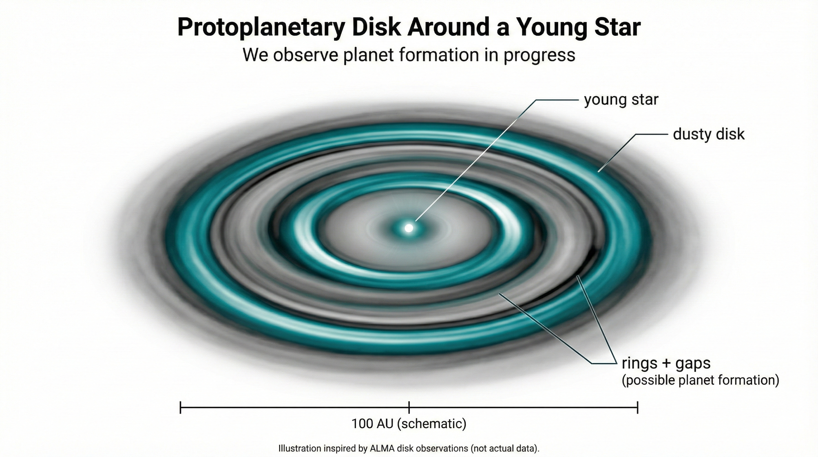
What to notice: we observe planet formation in progress — rings and gaps in young-star disks can be signatures of emerging planets. (Credit: (A. Rosen/Gemini — illustrative))
These disks aren’t relics — they’re active construction sites. The gaps and rings visible in disks around young stars (like HL Tau, observed by ALMA) are thought to be carved by forming planets. We’re watching the same process that built our solar system, playing out around other stars right now. In L12, we’ll shift from watching planets form to detecting the finished products.
Most planets orbit in the same plane and direction — but many moons are exceptions. Some moons are captured asteroids orbiting at odd angles (like Triton, which orbits Neptune backwards). Some moons formed from giant impacts (like Earth’s Moon).
The planet pattern supports the disk story. Moon orbits are messier because moons have additional formation pathways beyond the original disk.
If the solar system formed from a rotating disk of gas and dust, which of these would you expect to observe?
- Planets orbit in random directions at random angles
- All planets orbit in the same direction and nearly the same plane
- Inner planets orbit one direction, outer planets the other
- Planets don’t orbit at all — they should fly away
B) All planets orbit in the same direction and nearly the same plane. A rotating disk has a single spin direction and a flat geometry. Everything that forms from it inherits both properties. This is exactly what we observe — and it’s one of the strongest pieces of evidence for the nebular hypothesis.
Solar System Architecture:
- Rocky planets (Mercury–Mars) inside ~1.5 AU
- Gas giants (Jupiter, Saturn) at 5–10 AU
- Ice giants (Uranus, Neptune) at 19–30 AU
- Small bodies: asteroid belt, Kuiper Belt, Oort Cloud
Applying Our Toolkit:
- Masses from moon/spacecraft orbits (Newton’s gravity, L6)
- Temperatures from IR observations (Wien’s Law, L8)
- Compositions from spectral lines (L9)
- Everything connects back to Module 1!
Formation (The Causal Chain):
- Collapse \(\rightarrow\) spin-up \(\rightarrow\) disk \(\rightarrow\) temperature gradient \(\rightarrow\) condensation
- Angular momentum conservation explains disk formation and orbital patterns
- Frost line (~3 AU, model-dependent) explains rocky vs. gas giant distribution
Practice Problems
Solutions are available in the Lecture 11 Solutions.
Core (do these first)
1. Kepler Application: Mars orbits the Sun at 1.52 AU. Using Kepler’s Third Law (\(P^2 = a^3\) in Earth years and AU), calculate Mars’s orbital period.
2. Newton Application: Saturn’s moon Titan orbits at 1.22 million km with a period of 16 days. Estimate Saturn’s mass. (Compare to Jupiter’s mass from the worked example.)
3. Wien Application: Neptune’s thermal emission peaks at about \(50 \mu\mathrm{m}\) (50,000 nm). Estimate Neptune’s temperature using Wien’s Law.
4. Formation Concept: Explain why all the planets orbit the Sun in the same direction and in nearly the same plane.
5. Tool Choice: You want to determine whether a newly discovered exoplanet is rocky or gaseous. What two measurements would you need, and which tools from Module 1 would provide them?
Challenge
6. Frost Line Reasoning: If the Sun had been twice as luminous when the solar system formed, how would the frost line have been different? What consequences might this have for the distribution of planet types?
7. Integration Problem: You discover an exoplanet system where rocky planets extend out to 5 AU. What might this tell you about the host star compared to our Sun?
8. Frost Line from First Principles (Integration Problem): Equilibrium temperature scales with distance as \(T_{\text{eq}} \propto 1/\sqrt{a}\). Earth’s equilibrium temperature is ~255 K at 1 AU. Water ice condenses at ~150 K in the low-pressure solar nebula. Estimate the frost line distance.
9. Rocky or Gaseous? (Transfer Problem): You discover a new moon orbiting an exoplanet. From the moon’s orbit, you determine the planet’s mass is \(6.0 \times 10^{26}\) kg. From transit observations, you estimate the planet’s radius is \(6.0 \times 10^{7}\) m (about 9.4 \(R_\oplus\)). Calculate the planet’s average density. Is this planet more likely rocky or gaseous? Hint: Volume of a sphere = \(\frac{4}{3}\pi R^3\). Density = mass/volume.
10. Diagnosing a Mystery Planet (Multi-Tool Transfer): An infrared telescope detects thermal emission from a planet peaking at 20,000 nm (\(20 \mu\mathrm{m}\)). Spectroscopy of reflected starlight reveals strong \(\mathrm{CH_{4}}\) (methane) absorption lines but no \(CO_{2}.\) Is this planet more likely a rocky inner planet or an ice giant? Use Wien’s Law and your knowledge of atmospheric composition to justify your answer.
Glossary
- ★ Frost line
- The distance from the Sun (~3 AU) beyond which water ice could condense in the early solar nebula. Explains why rocky planets are close and gas/ice giants are far.
- ★ Gas giant
- A large planet composed primarily of hydrogen and helium; Jupiter and Saturn. No solid surface; formed beyond the frost line where more material was available.
- ★ Ice giant
- A large planet composed primarily of heavier volatiles (water, ammonia, methane); Uranus and Neptune. Distinguished from gas giants by their composition and smaller size.
- ◇ Kuiper Belt
- A region of icy bodies beyond Neptune, from ~30 to ~50 AU. Home to Pluto, Eris, and many other dwarf planets and comets.
- ★ Nebular hypothesis
- The theory that the solar system formed from a rotating disk of gas and dust around the young Sun. Explains common orbital direction, planetary spacing, and composition gradient.
- ◇ Oort Cloud
- A hypothetical spherical shell of icy objects at ~10,000–100,000 AU, the source of long-period comets. Never directly observed; inferred from comet orbits.
- ◇ Protoplanetary disk
- A rotating disk of gas and dust around a young star from which planets form. Observed around many young stars; confirms the nebular hypothesis.
- ★ Terrestrial planet
- A rocky planet with a solid surface; Mercury, Venus, Earth, and Mars in our solar system. Small, dense, close to the Sun; formed inside the frost line.