Module 1 Synthesis — Are We Alone?
Lecture 13 Reading Companion
You voted this your favorite NASA science question: Are we alone? Today we take it seriously — not as philosophy, but as astronomy. The Drake Equation provides a framework for estimating how many civilizations might exist in our galaxy. (We’ll zoom out to the observable universe later just for perspective — the numbers are staggering: up to \(\sim 10^{24}\) stars.) But the physics matters too: the earliest universe was metal-poor, so Earth-like rocky planets were unlikely at first. After the first generations of stars enriched the cosmos, rocky planets became possible. Stars had to create the ingredients first. This is why Module 2 — stellar evolution — is essential for understanding our place in the cosmos.
This is a synthesis lecture — shorter on new content, focused on integration and perspective.
Structure:
- Part 1: The Drake Equation — estimating cosmic company
- Part 2: Why the early universe was metal-poor (Module 2 preview)
- Part 3: Module 1 review and concept connections
Reading time: ~20 min (the lecture includes extended Q&A)
Exam prep: Part 3 summarizes all of Module 1. Use it as a study guide!
What’s next: Module 1 Exam on Monday. Then: Module 2 — Stars!
If you only remember three things:
Drake Equation: \(N = R_* \times f_p \times n_e \times f_l \times f_i \times f_c \times L\). The first three terms are now reasonably constrained; the last four remain complete mysteries.
The numbers are staggering: The Drake Equation applies to the Milky Way, but zooming out: up to \(\sim 10^{24}\) stars in the observable universe. Even tiny probabilities yield huge expected numbers — or, if we’re alone, the probability of life must be extraordinarily small.
Stars made the ingredients: The early universe was metal-poor. Rocky planets require heavy elements that stars created through fusion and dispersed through supernovae. Life requires stellar evolution.
Now for the details…
Your Favorite Question
At the start of the semester, we asked which of NASA’s big science questions interested you most. The winner, by a large margin: “Are we alone in the universe?”
It’s a question that has haunted humanity for millennia. But today we’re not going to approach it as philosophy or science fiction. We’re going to approach it as astronomy.
What would we actually need to calculate the answer? What do we know, what don’t we know, and what tools could help us find out?
In 1961, astronomer Frank Drake wrote down an equation — not to answer the question, but to organize our thinking about it. The Drake Equation breaks the question into pieces, each of which we can (in principle) estimate. Some terms we now know quite well. Others remain complete mysteries.
Along the way, we’ll encounter a key constraint: the earliest universe was metal-poor, so Earth-like rocky planets were unlikely at first. The ingredients — carbon, oxygen, silicon, iron — had to be created by stars and dispersed through supernovae. Understanding stellar evolution (Module 2) isn’t just about stars; it’s about understanding where we came from.
Let’s take your favorite question seriously.
Before we dive in, see if you can answer these from memory:
- L8: What determines whether a planet is in the habitable zone?
- L10: How does the radial velocity method detect exoplanets?
- L12: What is the transit depth, and what does it tell us?
- L9: What do spectral lines reveal about a star or planet?
- Distance from the star and stellar luminosity — where liquid water could exist
- The star wobbles due to the planet’s gravity, causing periodic Doppler shifts
- Transit depth = \((R_p/R_*)^2\) — it tells us the planet’s radius relative to the star
- Composition (which elements/molecules are present). If lines are shifted or broadened, they also reveal motion and physical conditions.
Part 1: The Drake Equation
A Framework for the Question
In 1961, radio astronomer Frank Drake convened a meeting to discuss the search for extraterrestrial intelligence (SETI). He wanted to organize the discussion, so he wrote down an equation that breaks the question into factors:
\[ N = R_* \times f_p \times n_e \times f_l \times f_i \times f_c \times L \]
where \(N\) = the number of communicating civilizations in our galaxy right now
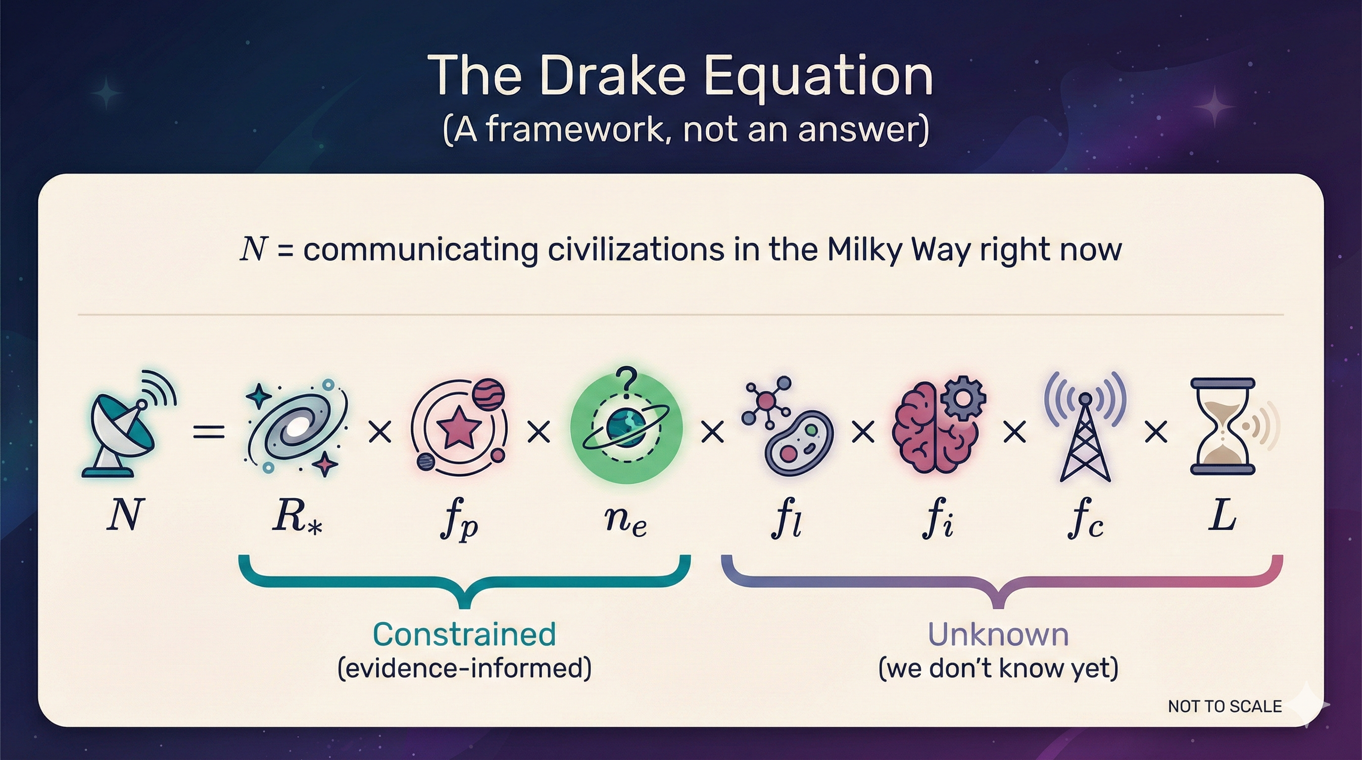
What to notice: The Drake Equation is a framework — a product of factors. The first few terms are astronomy-constrained; the later terms are still unknown. (Credit: (A. Rosen/Gemini — schematic))
The Terms
| Symbol | Meaning | What It Asks |
|---|---|---|
| \(R_*\) | Star formation rate | How many new stars per year? |
| \(f_p\) | Fraction with planets | How common are planetary systems? |
| \(n_e\) | Habitable planets per system | How many could support life? |
| \(f_l\) | Fraction that develop life | How often does life arise? |
| \(f_i\) | Fraction with intelligence | How often does intelligence evolve? |
| \(f_c\) | Fraction that communicate | How often do they build technology? |
| \(L\) | Civilization lifetime | How long do they last? |
The Power of the Framework
Drake didn’t expect to calculate an exact answer. The equation is a framework — it organizes what we need to know and reveals where our ignorance lies.
Some terms we now know fairly well (the first three). Others are complete guesses (the last four). Let’s work through them.
What We Know (Terms 1-3)
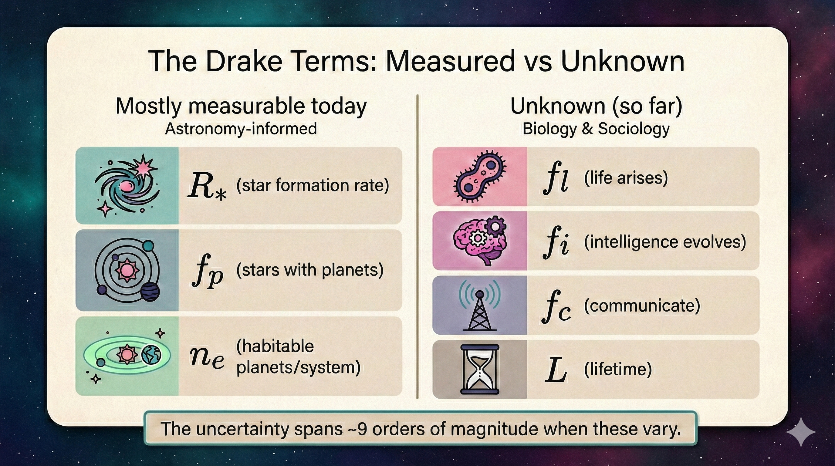
What to notice: Today, astronomy constrains \(R_*\), \(f_p\), and \(n_e\) reasonably well — but \(f_l\), \(f_i\), \(f_c\), and \(L\) remain unknown. (Credit: (A. Rosen/Gemini — schematic))
\(R_*\): Star Formation Rate
Question: How many new stars form in the Milky Way per year?
Answer: A few stars per year (order 1–10; often quoted as ~2–7 per year).
The exact number depends on how you convert the Milky Way’s star-formation rate (measured in solar masses per year) into individual stars using the initial mass function. This is well-established astrophysics — the uncertainty is mostly definitional, not observational.
\(f_p\): Fraction of Stars with Planets
Question: What fraction of stars have planetary systems?
Answer: On average, at least one planet for every star in the galaxy.
The Kepler mission (2009-2018) discovered thousands of exoplanets and showed that planets are the rule, not the exception. NASA/JPL now states that “on average, at least one planet for every star” — meaning \(f_p \approx 1\) is well-supported.
Module 1 connection: We find these planets using radial velocity (L10) and transits (L12).
\(n_e\): Habitable Planets per System
Question: On average, how many potentially habitable planets are there per planetary system?
Answer: Published estimates range from ~0.1 to ~0.5+ depending on definitions and star type.
This is less certain than \(f_p\). The number depends heavily on:
- What you mean by “Earth-like” (radius range)
- What you mean by “habitable zone” (conservative vs. optimistic)
- Which star types you consider (Sun-like vs. M dwarfs)
- Completeness corrections for detection biases
Some studies suggest ~22% of Sun-like stars host Earth-sized planets in the habitable zone; others find higher or lower values. The uncertainty is real — but it’s definitely not zero.
Module 1 connection: “Habitable” depends on stellar luminosity (L8 Stefan-Boltzmann), the habitable zone (L12), and atmospheric greenhouse effects (L12).
Which Drake Equation term has become MUCH better constrained in the last 20 years thanks to missions like Kepler?
- \(f_l\) (fraction that develop life)
- \(f_p\) (fraction of stars with planets)
- \(L\) (civilization lifetime)
- \(f_i\) (fraction with intelligence)
B) \(f_p\) (fraction of stars with planets). Before Kepler, we didn’t know if planets were common or rare. Now we know they’re ubiquitous — nearly every star has at least one planet. This was a major breakthrough in the 2010s.
Kepler and TESS also improved \(n_e\) (by finding Earth-sized planets in habitable zones), but they did NOT improve \(f_l\), \(f_i\), \(f_c\), or \(L\). Those remain completely unconstrained by exoplanet missions.
The Kepler mission found thousands of exoplanets. Which Drake Equation term is Kepler unable to constrain?
- \(f_p\) (fraction of stars with planets)
- \(n_e\) (habitable planets per system)
- \(f_l\) (fraction that develop life)
- \(R_*\) (star formation rate)
C) \(f_l\) (fraction that develop life). Kepler finds planets, not life. Finding a planet in the habitable zone doesn’t tell us whether life arose there. We have zero data points on \(f_l\) beyond Earth itself. This is why exoplanet discoveries, as exciting as they are, don’t resolve the Drake Equation — they only constrain the first few terms.
What We Don’t Know (Terms 4-7)
\(f_l\): Fraction That Develop Life
Question: Given a habitable planet, how often does life arise?
Answer: We have no idea.
We have exactly one example: Earth. Life arose here within a few hundred million years of conditions becoming suitable — which suggests it might be easy. But one example doesn’t tell us the probability.
If we found life on Mars (or Europa, or Enceladus), even microbial life, it would be revolutionary. Two independent origins in one solar system would suggest life is common.
\(f_i\): Fraction That Develop Intelligence
Question: Given life, how often does intelligence evolve?
Answer: Also unknown.
Life existed on Earth for ~3.5 billion years before intelligent, technological life emerged. Was that inevitable, or a lucky accident? We don’t know.
\(f_c\): Fraction That Communicate
Question: Given intelligent life, how often do they develop technology capable of interstellar communication?
Answer: Unknown.
Even on Earth, technologically advanced civilization has existed for only ~100 years (since radio). That’s 0.000003% of Earth’s history.
\(L\): Civilization Lifetime
Question: How long do technological civilizations last?
Answer: This is perhaps the most uncertain — and sobering — term.
Do civilizations destroy themselves (nuclear war, climate catastrophe, AI gone wrong)? Do they lose interest in communication? Do they spread throughout the galaxy and become undetectable?
\(L\) could be 100 years, 10,000 years, or millions of years. We don’t know.
The Drake Equation doesn’t give us an answer — it shows us what we need to learn.
Well-constrained: \(R_*\), \(f_p\), roughly \(n_e\)
Completely uncertain: \(f_l\), \(f_i\), \(f_c\), \(L\)
Depending on your assumptions, you can get \(N = 1\) (we’re alone) or \(N = 10,000+\) (the galaxy is teeming with civilizations). Both are consistent with current knowledge.
The equation’s value isn’t the answer — it’s the framework.
Three Drake Scenarios
Students learn uncertainty best by playing with the numbers. Here’s what happens when you vary the assumptions:
| Scenario | \(R_*\) | \(f_p\) | \(n_e\) | \(f_l\) | \(f_i\) | \(f_c\) | \(L\) (years) | N |
|---|---|---|---|---|---|---|---|---|
| Pessimistic | 3 | 1 | 0.2 | 0.01 | 0.01 | 0.01 | 100 | ~0.00006 |
| Middle | 3 | 1 | 0.2 | 0.1 | 0.1 | 0.1 | 10,000 | ~6 |
| Optimistic | 3 | 1 | 0.2 | 0.5 | 0.5 | 0.5 | 1,000,000 | ~75,000 |
The first three terms (\(R_*\), \(f_p\), \(n_e\)) are held constant at evidence-informed values. The last four terms (\(f_l\), \(f_i\), \(f_c\), \(L\)) are varied — and the result swings by nine orders of magnitude.
Note: \(N\) is an expected value (a statistical mean). If \(N \ll 1\), it means “probably zero, but not guaranteed.” If \(N = 6\), it means “we’d expect about 6 on average” — some galaxies might have more, some fewer.
That’s the power (and limitation) of the Drake Equation: it exposes where our ignorance lies.
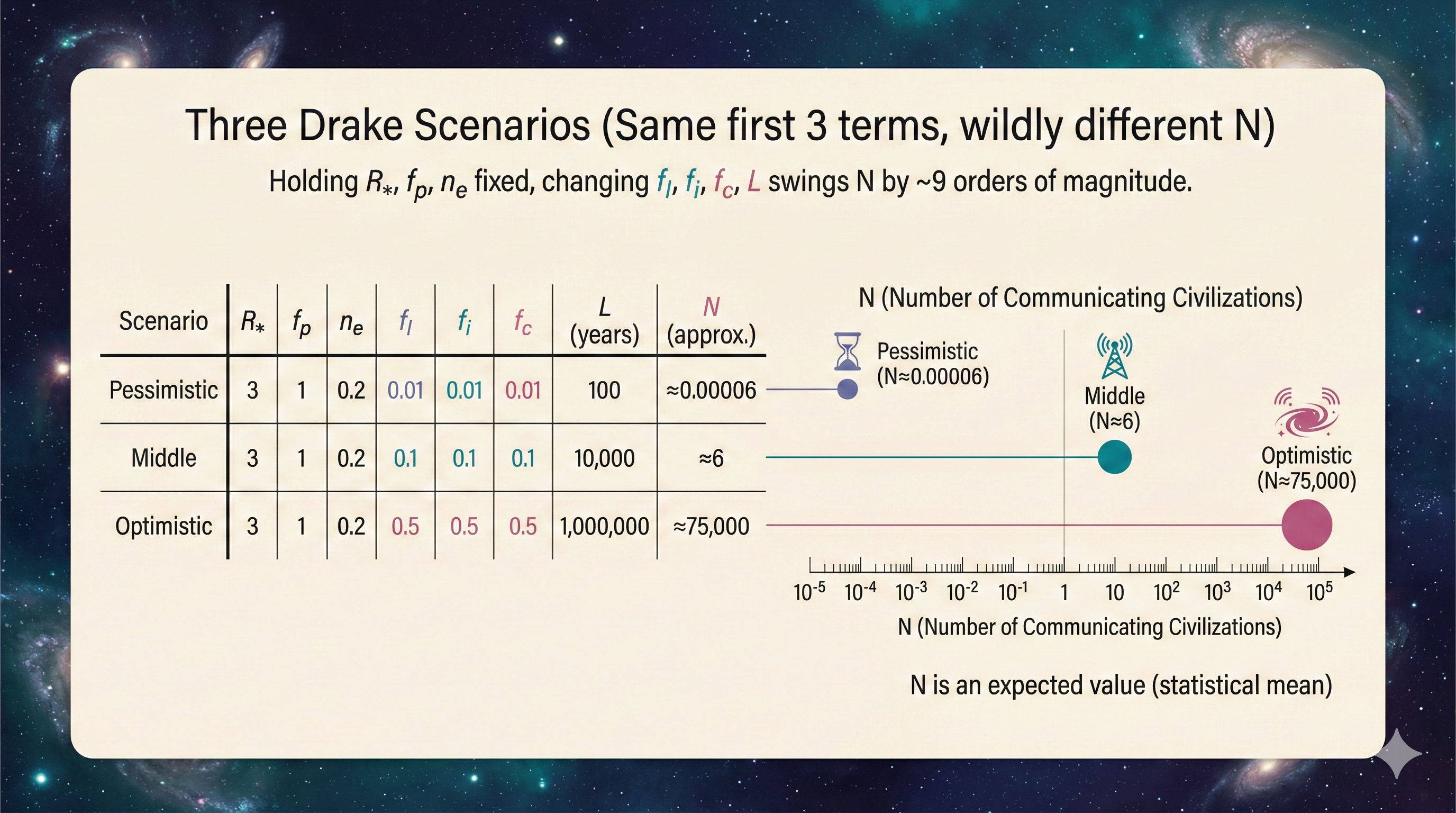
What to notice: Holding \(R_*\), \(f_p\), and \(n_e\) fixed, changing \(f_l\), \(f_i\), \(f_c\), and \(L\) can swing \(N\) by many orders of magnitude. The numbers shown are illustrative. (Credit: (A. Rosen/Gemini — schematic))
The Staggering Numbers
The Drake Equation is applied to the Milky Way. But to appreciate scale, let’s zoom out:
| Scale | Number |
|---|---|
| Stars in Milky Way | order \(10^{11}\) (roughly 100–400 billion) |
| Galaxies in observable universe | hundreds of billions to ~2 trillion |
| Total stars | up to \(\sim 10^{24}\) (a septillion!) |
That’s more stars than grains of sand on all of Earth’s beaches.
The probability argument:
If only one in a trillion trillion stars has intelligent life, the expected number would be ~1 — meaning the universe might have none, or it might have more; expectation doesn’t guarantee outcomes.
But if one in a billion has intelligent life, we’d expect \(\sim 10^{15}\) civilizations.
The universe is so vast that even tiny probabilities yield huge expected numbers. Or, if we’re truly alone, it means \(f_l \times f_i \times f_c \times L\) is extraordinarily small.
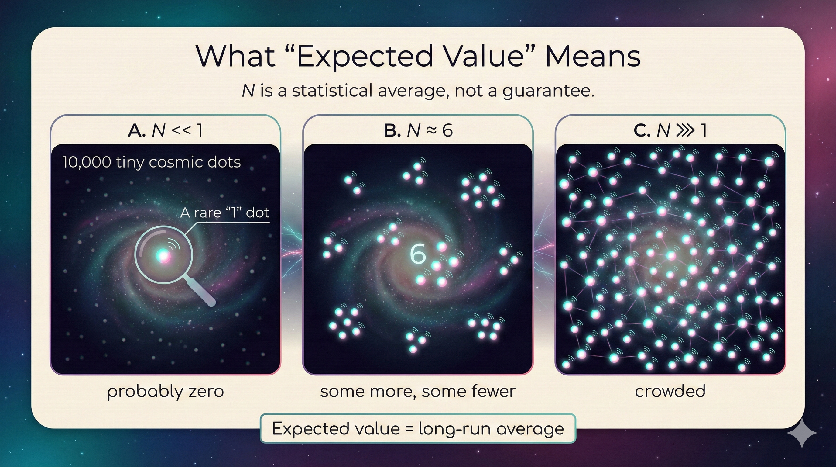
What to notice: \(N\) is an expected value — a long-run average, not a guarantee. Values like \(N \\ll 1\) can still produce rare ‘one-off’ cases. (Credit: (A. Rosen/Gemini — schematic))
The Fermi Paradox
In 1950, physicist Enrico Fermi asked: “Where is everybody?”
If the numbers are so large, and the universe is 13.8 billion years old, why haven’t we detected any signs of extraterrestrial intelligence?
Possible answers (we don’t know which is right):
- Intelligent life is extremely rare (\(f_l \times f_i \ll 1\))
- Civilizations don’t last long (\(L\) is small)
- They’re here but we haven’t noticed
- They’re not interested in communicating
- Interstellar travel/communication is harder than we think
- We haven’t looked hard enough yet
The Fermi Paradox remains one of the great unsolved puzzles. It reminds us that either we’re not alone (and something keeps us from detecting others) or we’re incredibly special.
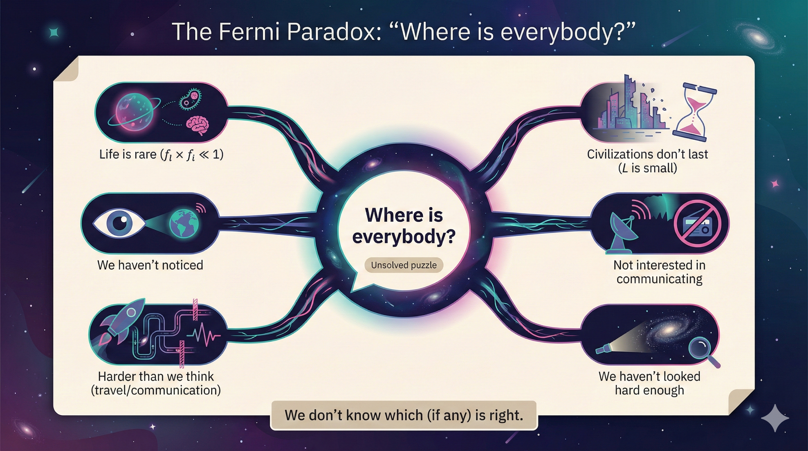
What to notice: The Fermi Paradox is the mismatch between ‘big expected numbers’ and ‘no detections yet.’ Multiple explanations are possible — we don’t know which (if any) is right. (Credit: (A. Rosen/Gemini — schematic))
Part 2: Why the Early Universe Was Metal-Poor
The Missing Ingredients
Here’s something we’ll explore deeply in Module 2: the early universe was almost entirely hydrogen and helium. Very little carbon. Very little oxygen. No silicon or iron to speak of.
These heavier elements — which astronomers call “metals” (even though that’s not the chemistry definition) — are essential for:
- Rocky planets (silicon, iron, oxygen)
- Complex chemistry (carbon, nitrogen, oxygen)
- Life as we know it (carbon-based molecules)
Where did the metals come from? Stars made them.
Metals (astronomy): Elements heavier than helium. This includes carbon, oxygen, iron — things chemists wouldn’t call “metals.”
Stars as Element Factories
Stars fuse light elements into heavier ones:
- Hydrogen \(\rightarrow\) Helium (main sequence stars, like the Sun)
- Helium \(\rightarrow\) Carbon, Oxygen (red giant stars)
- Carbon, Oxygen \(\rightarrow\) … \(\rightarrow\) Iron (massive stars)
- Elements heavier than iron (supernovae and neutron star mergers)
When stars die — especially massive stars that explode as supernovae — they scatter these elements into space. The next generation of stars (and planets) forms from this enriched material.
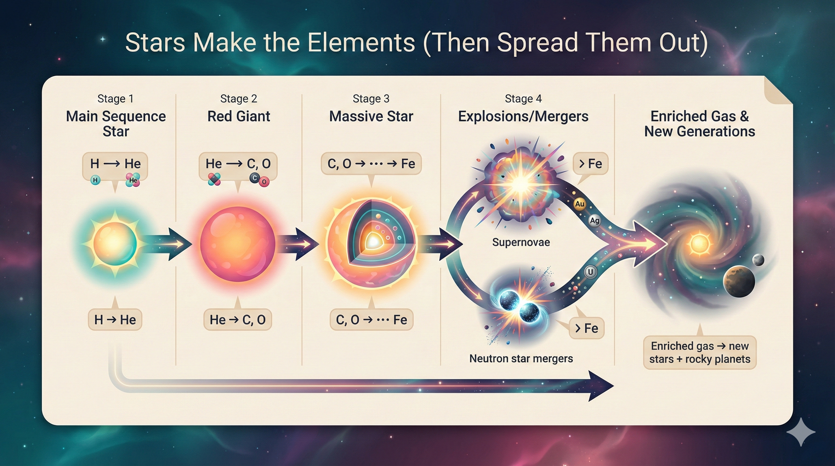
What to notice: Stars build the periodic table over generations. Fusion makes elements up to iron; supernovae and neutron star mergers make many heavier elements, enriching gas for later stars and rocky planets. (Credit: (A. Rosen/Gemini — schematic))
The Timeline
| Event | When | What Happened |
|---|---|---|
| Universe forms | 13.8 billion years ago | Almost entirely H and He |
| First stars form | As early as ~100 Myr after Big Bang (~13.7 Gyr ago) | Metal-free (Population III); rocky planets unlikely |
| First stars die | Shortly after | Enrich universe with metals via supernovae |
| Second-generation stars | ~13 billion years ago | Rocky planets become possible |
| Early rocky planets | ~11 billion years ago | Kepler-444 system shows rocky planets when universe was ~2.5 Gyr old |
| Sun forms | 4.6 billion years ago | Later-generation star, rich in metals for Earth |
The earliest universe was metal-poor, so Earth-like planets were unlikely at first. After the first generations of stars enriched the cosmos, rocky planets became possible — at least by a few billion years after the Big Bang, and maybe earlier. Exactly how early “habitable” worlds could exist is still an active research question.
Why were Earth-like rocky planets unlikely in the early universe?
- It was too hot
- There were no galaxies yet
- Heavy elements (metals) hadn’t been created yet
- Gravity was weaker
C) Heavy elements (metals) hadn’t been created yet. Rocky planets require silicon, iron, oxygen — elements that were scarce until the first generations of stars made them through nuclear fusion and dispersed them through supernovae. The early universe was almost entirely hydrogen and helium, so Earth-like worlds were unlikely until enrichment occurred.
Module 2 Preview
To understand where life can exist, we need to understand:
- How stars live and die (stellar evolution)
- How stars make heavy elements (nucleosynthesis)
- How long this process takes
- Which environments are favorable for planet formation
Module 2 isn’t “just” about stars — it’s about understanding the cosmic conditions for life. The search for life is deeply connected to stellar astrophysics.
Part 3: Module 1 Synthesis and Review
The Module 1 Toolkit
Everything we’ve learned connects to the search for life:
| Lecture | Key Tool | What It Reveals |
|---|---|---|
| L1-L2 | Scale of universe | Our cosmic context |
| L3-L4 | Celestial sphere, geometry | Positions, phases, eclipses |
| L5 | Kepler’s Laws | Orbital shapes, periods, distances |
| L6 | Newton’s Gravity | Why orbits work; mass from motion |
| L7 | EM Spectrum | Light as information carrier |
| L8 | Blackbody Radiation | Temperature from light (Wien, Stefan-Boltzmann) |
| L9 | Spectral Lines | Composition from light |
| L10 | Doppler Effect | Motion from light; exoplanets, dark matter |
| L11 | Solar System | Applying all tools to our neighborhood |
| L12 | Climate, Exoplanets | Greenhouse effect, transits, habitability |
| L13 | Drake Equation | Synthesizing the search for life |
The Concept Map
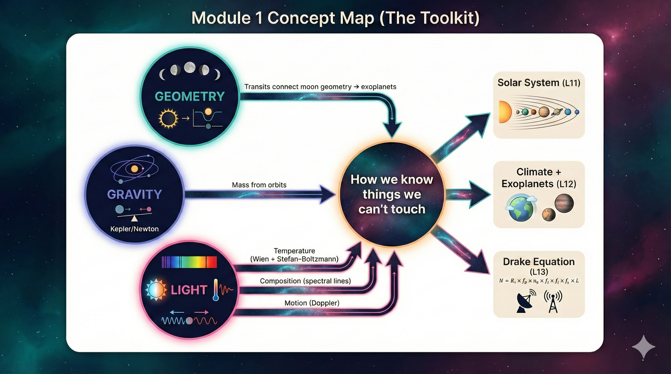
What to notice: Module 1’s toolkit (geometry, gravity, and light) is how we infer properties of worlds and stars we can’t touch — and it all feeds into exoplanets and the Drake Equation. (Credit: (A. Rosen/Gemini — schematic))
How everything connects:
LIGHT (L7-L10)
- Continuous spectrum \(\rightarrow\) Blackbody \(\rightarrow\) TEMPERATURE (L8)
- Stefan-Boltzmann \(\rightarrow\) Luminosity
- Wien’s Law \(\rightarrow\) Peak wavelength
- Spectral lines \(\rightarrow\) COMPOSITION (L9)
- Kirchhoff’s Laws
- Quantum energy levels
- Doppler shift \(\rightarrow\) MOTION (L10)
- Radial velocity
- Exoplanet detection
GRAVITY (L5-L6)
- Kepler’s Laws \(\rightarrow\) Orbital periods, distances
- Newton \(\rightarrow\) MASS from orbits
- Planet masses
- Dark matter
GEOMETRY (L3-L4)
- Celestial coordinates \(\rightarrow\) Positions
- Moon phases, eclipses \(\rightarrow\) Transit detection
ALL TOGETHER \(\rightarrow\) Solar system (L11), Climate (L12), Drake equation (L13)
Key Equations for the Exam
Kepler’s Third Law: \[ P^2 = a^3 \quad \text{(years, AU)} \] \[ P^2 = \frac{4\pi^2}{GM} a^3 \quad \text{(Newton's form)} \]
Stefan-Boltzmann Law: \[ L = 4\pi R^2 \sigma T^4 \]
Wien’s Law: \[ \lambda_{peak} = \frac{2.9 \times 10^6 \text{ nm}}{T} \]
Doppler Effect: \[ \frac{\Delta\lambda}{\lambda_0} = \frac{v}{c} \]
Hydrogen Energy Levels: \[ E_n = -\frac{13.6 \text{ eV}}{n^2} \]
Transit Depth: \[ \text{depth} = \left(\frac{R_p}{R_*}\right)^2 \]
Equilibrium Temperature: \[ T_{eq} = \left[ \frac{(1-A) L_\odot}{16\pi \sigma d^2} \right]^{1/4} \]
Common Exam Topics
Based on Module 1 content, be comfortable with:
Conceptual:
- Why planets/stars have the properties they have
- How we measure things we can’t touch (distance, mass, temperature, composition)
- Kirchhoff’s Laws — when do you get each type of spectrum?
- Why spectral lines appear at specific wavelengths (quantum)
- Doppler: what does it measure, what does it miss?
- Greenhouse effect and planetary climate
Quantitative:
- Using Kepler III to find period or distance
- Using Wien’s Law to find temperature
- Using Doppler formula to find velocity
- Using Stefan-Boltzmann conceptually (relative comparisons)
- Transit depth \(\rightarrow\) planet size
- Work practice problems — understanding comes from doing
- Explain concepts out loud — if you can’t explain it, you don’t understand it
- Connect the dots — how does L6 connect to L10? How does L8 connect to L12?
- Focus on “why” — not just formulas, but what they mean physically
The Drake Equation:
- \(N = R_* \times f_p \times n_e \times f_l \times f_i \times f_c \times L\)
- First three terms now reasonably known; last four remain uncertain
- Numbers are staggering: up to \(\sim 10^{24}\) stars in observable universe
- Fermi Paradox: If life is common, where is everybody?
Cosmic Context:
- Early universe: metal-poor — rocky planets unlikely at first
- Stars create heavy elements through fusion
- After first stellar generations enriched cosmos, rocky planets became possible
- Life requires stellar evolution — Module 2 is essential!
Module 1 Synthesis:
- Light reveals temperature, composition, motion
- Gravity and orbits reveal mass
- Geometry enables detection (transits, eclipses)
- All tools work together to explore the universe remotely
Practice Problems
Lecture 13 solutions are currently instructor draft and are not posted on the student site.
Core (do these first)
1. Drake Equation: If \(R_* = 3\)/year, \(f_p = 1\), \(n_e = 0.2\), and we assume all remaining factors equal 1, how many civilizations are currently in our galaxy? What’s unrealistic about this assumption?
2. Synthesis Question: A star’s spectrum shows: (a) a blackbody peak at 500 nm, and (b) absorption lines shifted 0.1% toward longer wavelengths. What can you determine about this star from each observation?
3. Early Universe: Explain why Earth-like rocky planets were unlikely in the early universe. What had to happen first?
4. Tool Identification (Synthesis): For each measurement below, identify which Module 1 tool or law provides it: (a) a star’s surface temperature, (b) whether a star is approaching or receding, (c) a planet’s radius, (d) a planet’s orbital period from radial velocity data, (e) the total mass enclosed within a galaxy at a given radius.
Challenge
5. Full Synthesis: You detect an exoplanet via both radial velocity (amplitude 50 m/s, period 10 days) and transit (depth 0.5%). The host star is Sun-like. What can you determine about the planet? List each property and which observation/method gives it.
6. Drake Sensitivity: In the Drake Equation, the “middle” scenario uses \(f_l = f_i = f_c = 0.1\) and \(L = 10{,}000\) years (with \(R_* = 3\), \(f_p = 1\), \(n_e = 0.2\)), giving \(N \approx 6\). If civilizations last \(10\times\) longer (\(L = 100{,}000\) years) but intelligence is \(10\times\) rarer (\(f_i = 0.01\)), does \(N\) change? What does this tell you about the structure of the Drake Equation?
7. Habitable Zone + Wien’s Law Integration: A star’s spectrum peaks at 350 nm. (a) Use Wien’s Law (\(b = 2.9 \times 10^6\) \(nm\cdot K)\) to find its surface temperature. (b) Assuming the star has the same radius as the Sun, use \(L \propto T^4\) to estimate its luminosity relative to the Sun (\(T_\odot = 5800\) K). (c) The habitable zone scales as \(\sqrt{L/L_\odot}\) in AU — where is this star’s habitable zone compared to Earth’s orbit?
8. Fermi Paradox: The Milky Way has been forming stars for ~13 billion years; the Sun formed ~4.6 billion years ago. Estimate how much “head start” an alien civilization around an older star could have on us. What might they have accomplished in that time?
Glossary
- ◇ Abiogenesis
- The natural process by which life arises from non-living matter. How common is this? We have one example (Earth) and don't know the probability.
- ★ Biosignature
- A detectable sign of life, such as atmospheric gases (O₂, CH₄) that are unlikely without biological processes. A key target for future telescope observations of exoplanet atmospheres.
- ★ Drake Equation
- A framework for estimating the number of communicating civilizations in the galaxy: N = R* × fp × ne × fl × fi × fc × L. Not a calculation but a way to organize our ignorance about astrobiology.
- ★ Fermi Paradox
- The apparent contradiction between the high probability of extraterrestrial civilizations and the lack of evidence for them. 'Where is everybody?' — Enrico Fermi, 1950.
- ◇ Great Filter
- A hypothetical barrier in the evolution of life that makes advanced civilizations extremely rare. Could be in our past (we passed it) or our future (we haven't reached it yet).
- ◇ SETI
- Search for Extraterrestrial Intelligence; the scientific effort to detect signals from alien civilizations. Primarily searches for artificial radio or optical signals.
Module 1 Self-Assessment
Before the exam, can you:
☐ Explain Kepler’s Three Laws and use the third law to find periods/distances?
☐ Apply Newton’s gravity to find mass from orbital motion?
☐ Describe the electromagnetic spectrum and atmospheric windows?
☐ Use Wien’s Law to find temperature from peak wavelength?
☐ Use Stefan-Boltzmann conceptually (how does L change with T and R)?
☐ Explain Kirchhoff’s Laws and when each type of spectrum occurs?
☐ Explain why spectral lines are discrete (quantum energy levels)?
☐ Apply the Doppler formula to find radial velocity?
☐ Explain how RV method detects exoplanets?
☐ Explain what transits measure and how?
☐ Describe the greenhouse effect and why Venus/Earth/Mars differ?
☐ Explain why the early universe was metal-poor and rocky planets were unlikely at first?
If you can do all of these, you’re ready. If not, review those topics!
What’s Next
Monday (Mar 2): Module 1 Exam
Then: Module 2 — Stars!
We’ll learn how stars are born, how they live, and how they die. We’ll understand why massive stars explode and where the elements in your body came from. Stellar evolution isn’t just about stars — it’s about understanding the universe’s chemical evolution and the conditions for life.
See you in Module 2!