Planetary Climates & Finding Other Worlds
Lecture 12 Reading Companion
Planet climates are an energy-balance problem. Sunlight in, infrared out. Equilibrium temperature is the baseline; atmospheres (greenhouse gases, clouds, pressure) push real surface temperatures above or below that baseline. The same physics that explains Venus, Earth, and Mars is what we use to judge exoplanet habitability — after we find those planets using transits and radial velocity.
This reading has two main parts:
Part 1: Planetary Climates (~25 min)
- Why planetary temperatures differ from simple predictions
- The greenhouse effect explained
- Venus vs. Earth vs. Mars: what went wrong/right
- Climate change connection
Part 2: Exoplanet Detection (~20 min)
- Transit method (geometry callback to L4!)
- Combining with radial velocity (L10)
- The habitable zone
Exam connection: This lecture reinforces L8 (blackbody/Stefan-Boltzmann) and L10 (Doppler). Climate physics applies thermal equilibrium. Transit detection applies geometry from L4.
What’s next: L13 asks the big question: Are we alone? We’ll use the Drake Equation to estimate how many civilizations might exist.
If you only remember three things:
Greenhouse effect: Atmospheres absorb some outgoing infrared, warming the surface above equilibrium. Venus = extreme (+500 K), Earth = moderate (+33 K), Mars = minimal (+8 K).
Transits detect exoplanets: When a planet crosses its star, brightness dips by \((R_p/R_*)^2\). Combined with radial velocity \(\rightarrow\) mass + radius \(\rightarrow\) density \(\rightarrow\) rocky or gaseous?
Habitable zone: Where liquid water could exist. Depends on stellar luminosity and planetary atmosphere. Zone \(\ne\) guarantee!
Now for the details…
Three Worlds, Three Fates
Venus, Earth, and Mars are siblings — rocky planets that formed from the same solar nebula about 4.6 billion years ago. You might expect similar conditions. Instead, we find three radically different worlds:
Venus: Surface temperature 735 K (\(462^{\circ}\)C) — hot enough to melt lead. Crushing atmospheric pressure \(90\times\) Earth’s. Sulfuric acid clouds. No liquid water. A hellscape.
Earth: Surface temperature 288 K (\(15^{\circ}\)C). Moderate atmosphere. Liquid water oceans covering 70% of the surface. Life everywhere, from deep ocean vents to Antarctic ice.
Mars: Surface temperature 218 K (-\(55^{\circ}\)C). Atmospheric pressure less than 1% of Earth’s. Frozen polar caps. Ancient river channels, but no liquid water today. A cold desert.
What explains these vastly different outcomes? The answer involves physics we’ve already learned: blackbody radiation, thermal equilibrium, and atmospheric absorption. Today we’ll see how the greenhouse effect creates these different climates — and why adding \(\mathrm{CO_{2}}\) to Earth’s atmosphere shifts the same energy balance (though in a vastly different regime than Venus).
Then we’ll turn to the search for other worlds. We’ve found thousands of exoplanets, some in “habitable zones” where liquid water could exist. How do we find them? And what determines if they’re actually habitable?
Before we dive in, see if you can answer these from memory:
- L8: What law relates an object’s temperature to the total power it radiates per unit area?
- L8: If an object’s temperature doubles, by what factor does its radiated power increase?
- L10: When a star moves toward us, are its spectral lines blueshifted or redshifted?
- L4: Why don’t we see a solar eclipse every month?
- Stefan-Boltzmann Law
- \(16\times\) (since P \(\propto\) \(T^{4})\)
- Blueshifted
- Moon’s orbit is tilted ~\(5^{\circ}\) relative to the ecliptic — alignment is rare
Part 1: Planetary Climates
Equilibrium Temperature — A First Guess
In L8, we learned that objects in thermal equilibrium absorb and emit energy at equal rates. For a planet absorbing sunlight:
\[ \text{Energy absorbed} = \text{Energy emitted} \]
This gives an equilibrium temperature — what the planet’s temperature should be if it’s just balancing incoming sunlight against outgoing thermal radiation.
Equilibrium temperature: The temperature a planet would have if it only balanced absorbed sunlight against blackbody emission, with no atmospheric effects.
Deep Dive: Deriving Equilibrium Temperature
Let’s work through the calculation step by step.
Step 1: Energy Balance
At equilibrium, energy in equals energy out:
\[ \text{Power absorbed from Sun} = \text{Power radiated to space} \]
We already know the right side from L8: a blackbody radiates power according to the Stefan-Boltzmann Law:
\[ P_{out} = \sigma T^4 \times (\text{surface area}) \]
This is the key connection! The Stefan-Boltzmann Law from L8 tells us how much power a planet radiates at temperature T. Setting this equal to absorbed sunlight gives us the equilibrium temperature.
But how much solar power does a planet actually intercept?
Step 2: Why \(\pi R^2\), Not \(4\pi R^2\)? — The Disk Approximation
Here’s a key insight: A planet doesn’t absorb sunlight over its entire spherical surface. Sunlight comes from one direction (the Sun), so the planet only intercepts light across its cross-sectional area — the area of the “shadow” it would cast.
During a total solar eclipse, the Moon blocks the Sun. But the Moon’s shadow on Earth isn’t sphere-shaped — it’s a disk. That’s because sunlight travels in parallel rays from the distant Sun, and the Moon intercepts them with its cross-sectional area.
Cross-section of a sphere = \(\pi R^2\) (the area of a circle with the same radius)
The planet intercepts sunlight like a disk \((\pi R^2)\) but radiates from its entire spherical surface \((4\pi R^2)\). This factor of 4 difference is crucial for the calculation!
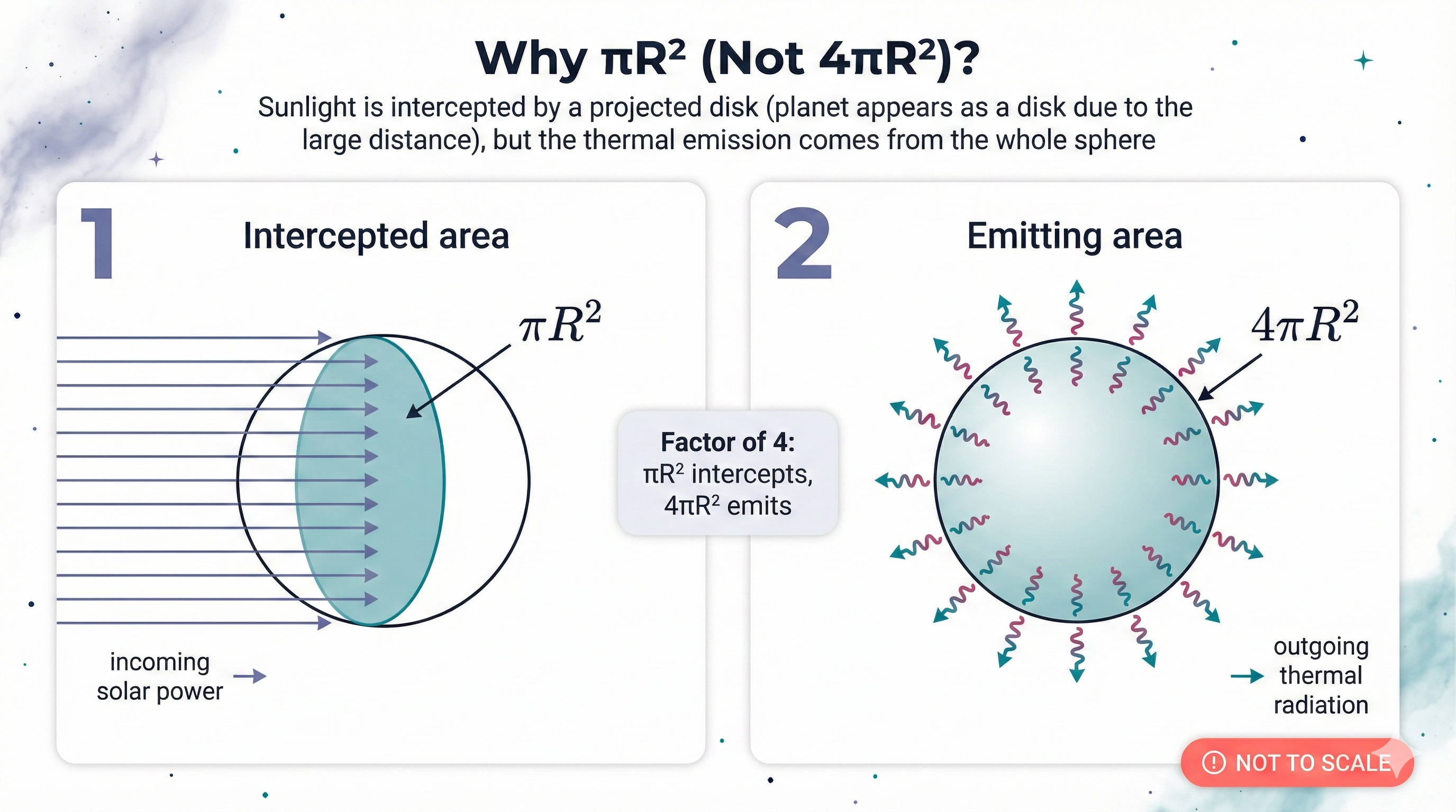
What to notice: a planet intercepts sunlight over its projected disk (πR²) but emits thermal radiation from its whole surface (4πR²) — that factor of 4 is why equilibrium temperatures use 16π in the denominator. (Credit: (A. Rosen/Gemini — schematic))
Step 3: What Is Albedo?
Not all sunlight that hits a planet gets absorbed — some reflects back into space. Albedo (A) is the fraction of incoming light that reflects away.
- Albedo = 0 \(\rightarrow\) perfectly absorbing (all light absorbed)
- Albedo = 1 \(\rightarrow\) perfectly reflecting (all light bounces off)
- Real planets: somewhere in between
These are Bond albedos — the fraction of total incoming energy reflected, averaged over all wavelengths and angles. (Geometric albedo, which you may see elsewhere, measures reflectivity at a single viewing angle.)
| Body | Bond Albedo | Why? |
|---|---|---|
| Venus | ~0.76 | Thick, bright sulfuric-acid clouds reflect most light |
| Earth | ~0.30 | Mix of clouds, oceans (dark), ice (bright) |
| Mars | ~0.25 | Dusty, rocky surface with thin atmosphere |
| Moon | ~0.11 | Dark basalt surface, no atmosphere |
Albedo (Bond): The fraction of total incoming energy reflected back to space, averaged over all wavelengths and angles. Used for energy-balance calculations.
If a planet reflects fraction A, it absorbs fraction (1 - A).
- Venus absorbs only 25% of incoming sunlight
- Earth absorbs 70%
- Mars absorbs 75%
Venus has the highest albedo of these planets — it reflects most of its sunlight! This should make it cooler than Earth. The fact that Venus is instead the hottest planet in the solar system (even hotter than Mercury) tells you how powerful its greenhouse effect is.
Venus reflects 76% of incoming sunlight. Earth reflects 30%. Based only on albedo (ignoring distance), which planet absorbs more solar energy?
- Venus — it’s closer to the Sun
- Earth — it absorbs 70% vs. Venus’s 24%
- They absorb the same amount
- Can’t tell without knowing their sizes
B) Earth absorbs a larger fraction of incident sunlight — 70% vs. Venus’s 24%. Venus absorbs only about a quarter of the sunlight hitting it, while Earth absorbs nearly three-quarters. Of course, Venus receives more total sunlight (closer to the Sun), so the full picture requires the equilibrium temperature formula below. But the albedo alone would make Venus cooler!
Step 4: Putting It All Together
Now we can set up the full energy balance:
Power absorbed:
\[ P_{in} = (\text{Solar flux at planet}) \times (\text{cross-section}) \times (1 - A) \]
The solar flux at distance \(d\) from the Sun is:
\[ F = \frac{L_\odot}{4\pi d^2} \]
So:
\[ P_{in} = \frac{L_\odot}{4\pi d^2} \times \pi R^2 \times (1 - A) \]
Power radiated:
\[ P_{out} = \sigma T_{eq}^4 \times 4\pi R^2 \]
Setting them equal:
\[ \frac{L_\odot}{4\pi d^2} \times \pi R^2 \times (1 - A) = \sigma T_{eq}^4 \times 4\pi R^2 \]
Notice that \(\pi R^2\) appears on both sides — the planet’s size cancels out! This is why equilibrium temperature doesn’t depend on planet size.
Solving for \(T_{eq}\):
\[ T_{eq} = \left[ \frac{(1-A) L_\odot}{16\pi \sigma d^2} \right]^{1/4} \]
Looking at the formula:
\[ T_{eq} = \left[ \frac{(1-A) L_\odot}{16\pi \sigma d^2} \right]^{1/4} \]
The equilibrium temperature depends on:
- Distance (d): Farther \(\rightarrow\) lower T_eq (goes as \(d^{-1/2}\))
- Albedo (A): Higher albedo \(\rightarrow\) lower T_eq (absorbs less)
- Stellar luminosity (L): Brighter star \(\rightarrow\) higher T_eq
It does NOT depend on:
- Planet radius (canceled out!)
- Planet mass
- Whether the planet has an atmosphere (that comes later!)
Equilibrium temperature is a model, not a measurement.
\(T_{eq}\) is what a bare, airless sphere would have if it only balanced absorbed sunlight against blackbody emission. Real surface temperatures differ because:
- Atmospheres trap heat (greenhouse effect)
- Planets rotate, redistributing heat
- Internal heat sources (e.g., Jupiter radiates more than it absorbs)
When you see a planet’s “temperature” in the news, ask: equilibrium, effective, or surface? They’re different numbers.
Simplified Formula for Quick Estimates
For a perfectly absorbing planet (A = 0) orbiting the Sun:
\[ T_{eq} \approx 279\text{ K} \times \left(\frac{1\text{ AU}}{d}\right)^{1/2} \]
To correct for albedo, multiply by \((1-A)^{1/4}\):
\[ T_{eq} \approx 279\text{ K} \times (1-A)^{1/4} \times \left(\frac{1\text{ AU}}{d}\right)^{1/2} \]
Sanity check for Earth (d = 1 AU, A \(\approx\) 0.30):
\[ T_{eq} \approx 279 \times (0.70)^{1/4} \approx 279 \times 0.91 \approx 255\text{ K} \]
That matches the table below — and it’s about 33 K colder than Earth’s actual surface temperature. The difference? The greenhouse effect.
The Predictions vs. Reality
| Planet | Distance (AU) | T_equilibrium (K) | T_actual (K) | Difference |
|---|---|---|---|---|
| Venus | 0.72 | ~230 | 735 | +505 K ⚠️ |
| Earth | 1.00 | ~255 | 288 | +33 K |
| Mars | 1.52 | ~210 | 218 | +8 K |
Something is very wrong with our prediction for Venus. It’s 500 degrees hotter than equilibrium! Earth is also warmer than expected, but by a modest 33 K. What’s going on?
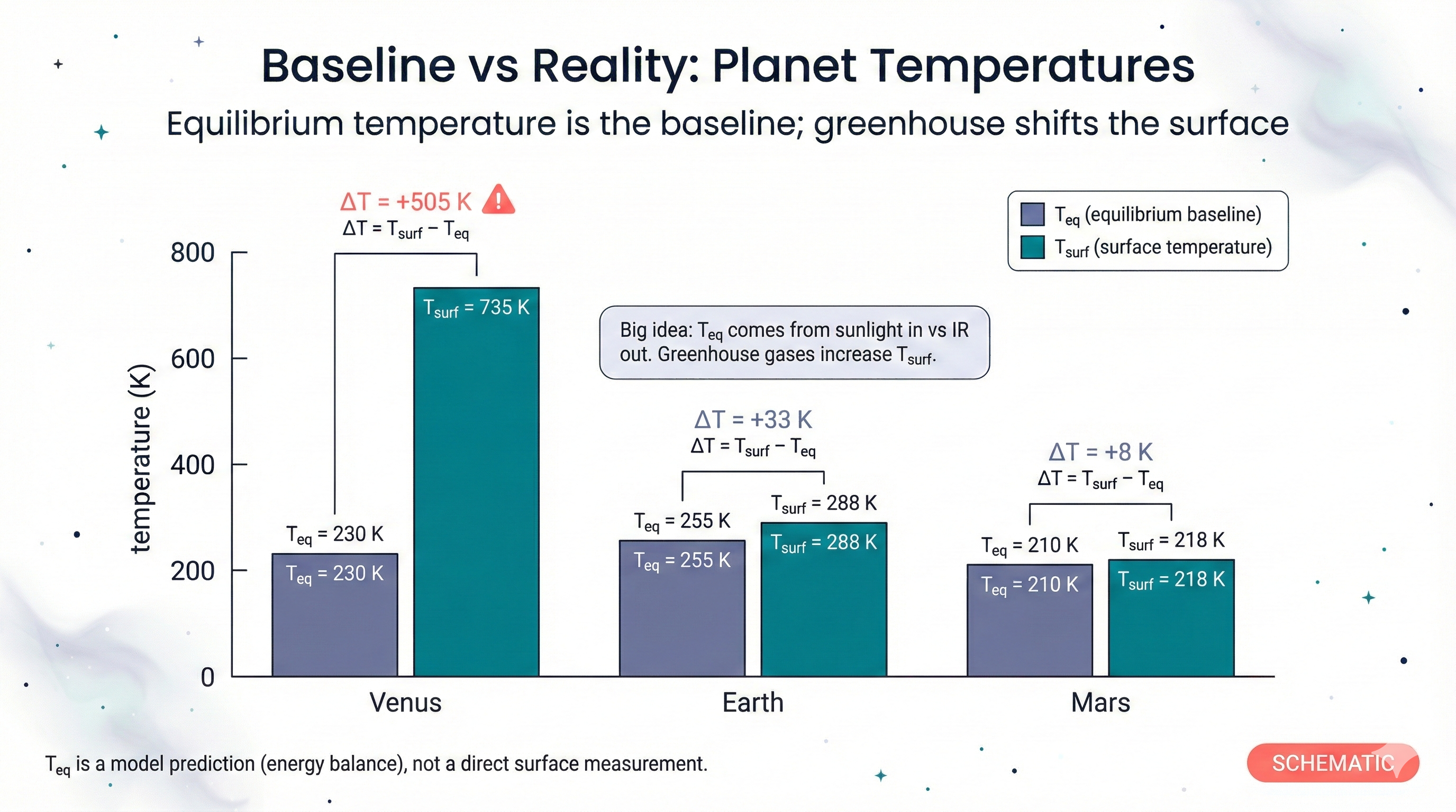
What to notice: equilibrium temperature is a baseline from sunlight-in vs IR-out; greenhouse physics shifts the real surface temperature above that baseline by different amounts on Venus, Earth, and Mars. (Credit: (A. Rosen/Gemini — schematic))
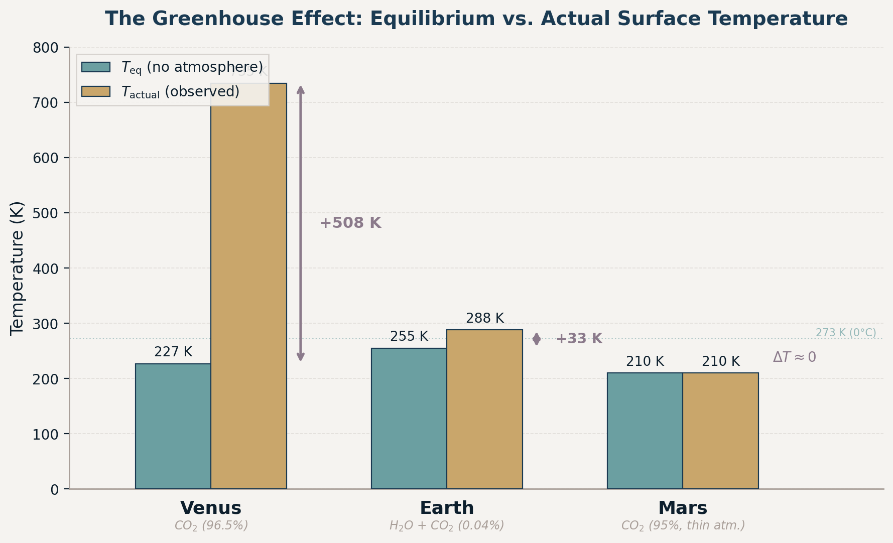
What to notice: Venus, Earth, and Mars start at similar equilibrium temperatures (set by distance and albedo), but the greenhouse effect adds vastly different amounts of warming — over 500 K for Venus, 33 K for Earth, and only 8 K for Mars. (Credit: ASTR 201 (generated))
Observable: Venus radiates thermally at 735 K in the infrared. (Wavelength + Brightness)
Model: Equilibrium temperature from distance and albedo predicts only ~230 K.
Inference: Something is adding +505 K beyond what sunlight alone explains. The culprit: a massive CO\(_2\) greenhouse effect. The gap between prediction and observation is itself the evidence.
Based only on distance from the Sun, which planet should be warmest?
- Venus
- Earth
- Mars
- They should all be the same temperature
A) Venus. Closer to the Sun means more intense sunlight, so a higher equilibrium temperature. But Venus’s actual temperature is even higher than this prediction — that’s where the greenhouse effect comes in.
The Greenhouse Effect
The Basic Mechanism
The equilibrium calculation assumes the planet radiates directly to space. But if the planet has an atmosphere containing greenhouse gases, something different happens:
Sunlight (visible) passes through the atmosphere and heats the surface
The surface emits infrared radiation (thermal, from Wien’s Law)
Greenhouse gases selectively absorb infrared — they’re transparent to visible light but absorb in key IR wavelength bands
The atmosphere re-radiates — some back down to the surface
The effective emission level moves higher in the atmosphere — where it’s colder. To radiate the same total power to space, the surface must warm up to compensate. (Think of it this way: the atmosphere acts like a blanket, so the skin under the blanket has to be warmer to maintain the same heat flow outward.)
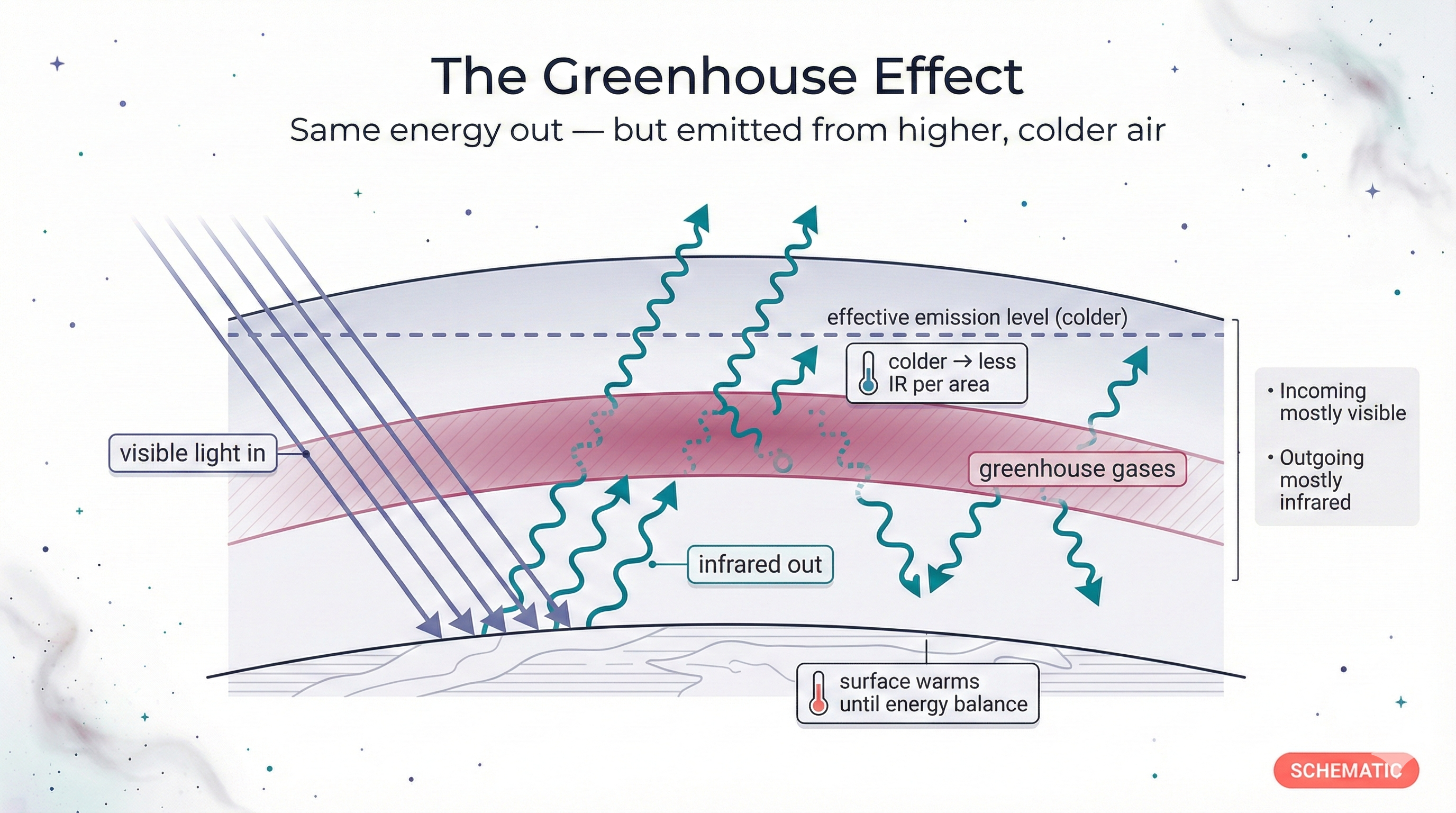
What to notice: the same energy must leave to space, but greenhouse gases shift the effective emission level upward to colder air, so the surface warms until energy balance is restored. (Credit: (A. Rosen/Gemini — schematic))
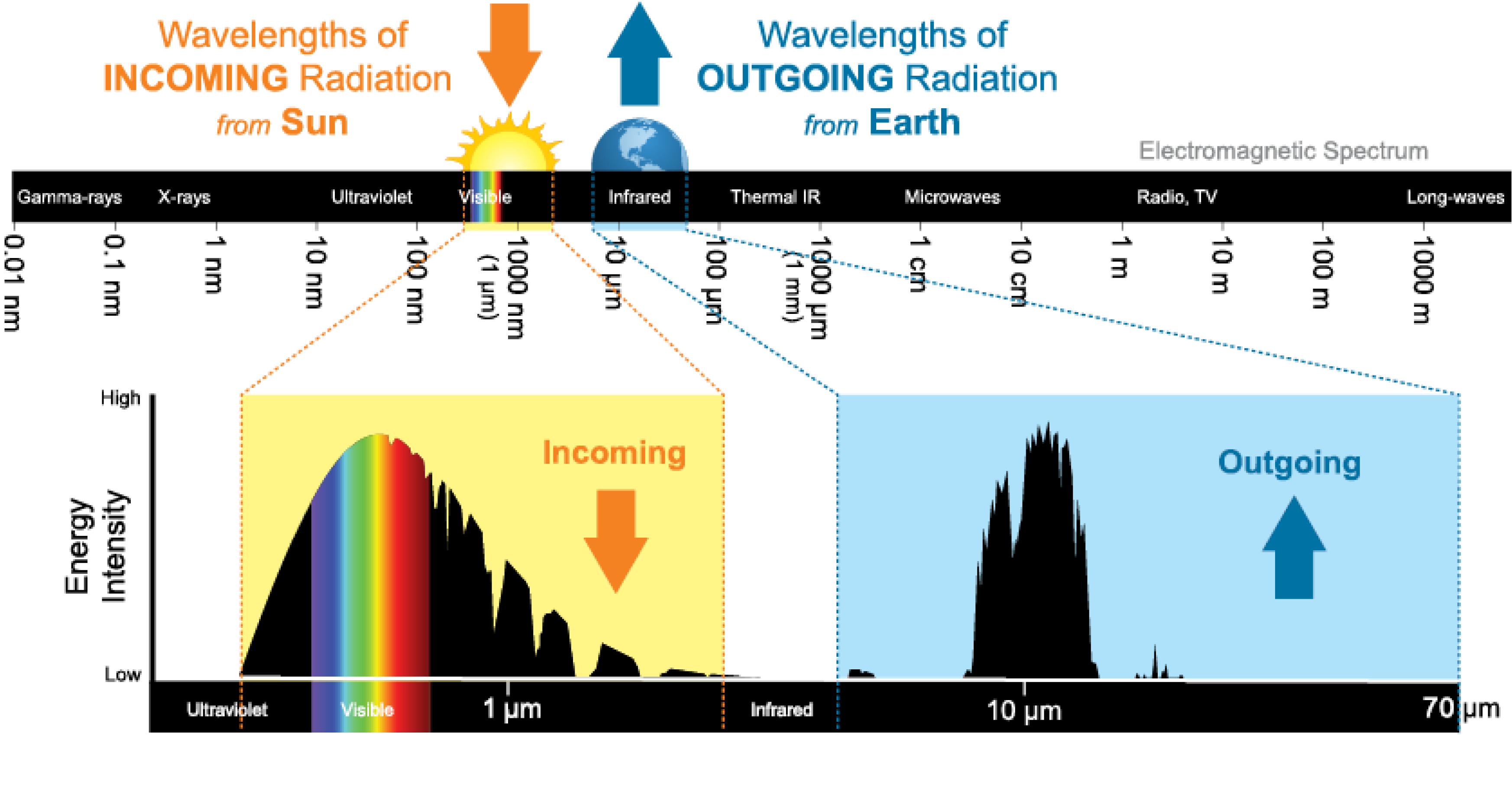
What to notice: the Sun’s emission peaks in visible light (short wavelength), while Earth’s emission peaks in the infrared (long wavelength). Greenhouse gases absorb selectively in the infrared, which is why the atmosphere is transparent to sunlight but opaque to Earth’s thermal emission. (Credit: NOAA JetStream)
Key Greenhouse Gases
| Gas | Chemical Formula | Effect |
|---|---|---|
| Water vapor | \(\mathrm{H_{2}O}\) | Strong absorber; amplifies other effects |
| Carbon dioxide | \(\mathrm{CO_{2}}\) | Primary driver; very long-lived |
| Methane | \(\mathrm{CH_{4}}\) | Potent but shorter-lived |
| Nitrous oxide | \(\mathrm{N_{2}O}\) | Long-lived, potent |
Why do greenhouse gases absorb infrared specifically?
From Wien’s Law: \(\lambda_{\text{peak}} = 2.9 \times 10^6 /T\) nm
- Sun (5800 K): Peak at ~500 nm (visible) \(\rightarrow\) passes through atmosphere
- Earth (288 K): Peak at ~10,000 nm (infrared) \(\rightarrow\) absorbed by greenhouse gases
The atmosphere is largely transparent to incoming visible light but selectively absorbs outgoing infrared in key wavelength bands. That’s the essence of the greenhouse effect!
Venus — Runaway Greenhouse
What Went Wrong on Venus?
Venus may have started with conditions similar to Earth — perhaps even with liquid water oceans. But it was closer to the Sun, so it was warmer. Here’s what may have happened:
Higher temperature \(\rightarrow\) more water evaporates
Water vapor is a greenhouse gas \(\rightarrow\) temperature rises further
More evaporation \(\rightarrow\) more water vapor \(\rightarrow\) more warming (positive feedback!)
Eventually: oceans boil completely
UV light breaks apart water vapor \(\rightarrow\) hydrogen escapes to space
\(\mathrm{CO_{2}}\) from volcanoes accumulates (no oceans to dissolve it, no life to sequester it)
Result: 96% \(\mathrm{CO_{2}}\) atmosphere, 735 K surface
The Runaway Greenhouse
This is a runaway greenhouse effect — a positive feedback loop where warming causes more warming until a new, much hotter equilibrium is reached.
Venus’s atmosphere is now 96% \(\mathrm{CO_{2}}\) with \(90\times\) Earth’s surface pressure. The greenhouse effect adds over 500 K to its temperature.
How do we know Venus’s surface conditions so precisely? Because we’ve landed on it. The Soviet Venera missions (1970s-80s) were the first spacecraft to land on another planet and return data. Venera 13 survived 127 minutes on Venus’s surface in 1982 — enduring 735 K heat and 90 atmospheres of pressure — long enough to take the first color photos of Venus’s surface and analyze the soil.
The photos reveal a flat, rocky landscape under an orange sky (the thick atmosphere scatters blue light away). Every Venera lander was eventually crushed by the pressure, but the data they returned confirmed the extreme greenhouse diagnosis.
Venus shows what happens when the greenhouse effect runs away.
The same radiative physics governs all planetary climates — but Earth and Venus occupy vastly different regimes. Earth is not on a trajectory toward Venus-style runaway; our solar flux is too low and our oceans act as a \(\mathrm{CO_{2}}\) buffer. What is happening: adding greenhouse gases shifts Earth’s energy balance, raising surface temperatures by degrees, not hundreds of degrees. Small shifts still have large consequences.
Venus is hotter than Mercury, even though Mercury is closer to the Sun. Why?
- Venus has a stronger magnetic field
- Venus has a thick \(\mathrm{CO_{2}}\) atmosphere causing a strong greenhouse effect
- Venus rotates more slowly
- Venus has active volcanoes
B) Venus has a thick \(\mathrm{CO_{2}}\) atmosphere causing a strong greenhouse effect. Mercury has almost no atmosphere, so it experiences huge day–night temperature swings (~700 K dayside, ~100 K nightside) with no greenhouse warming. Venus’s thick \(\mathrm{CO_{2}}\) atmosphere traps heat uniformly, raising the surface to ~735 K everywhere — hotter than Mercury’s dayside despite being farther from the Sun.
Mars — Too Little Atmosphere
Why Mars Is Cold
Mars has the opposite problem: its atmosphere is too thin to trap much heat.
- Surface pressure: 0.6% of Earth’s
- Composition: 95% \(CO_{2},\) but so thin it barely matters
- Result: Only ~8 K of greenhouse warming
Mars also lost much of its early atmosphere. With weak gravity (38% of Earth’s) and no global magnetic field, the solar wind stripped away atmospheric gases over billions of years.
Evidence of Past Water
Mars wasn’t always this way. We see:
- Ancient river channels and lake beds
- Minerals that only form in liquid water
- Polar ice caps \((CO_{2}\) and water ice)
Early Mars may have had a thicker atmosphere and liquid water. Climate change — going the opposite direction from Venus — froze and dried the planet.
Mars has 95% CO\(_2\) in its atmosphere — the same gas that makes Venus a hellscape. Why doesn’t Mars have a strong greenhouse effect?
- Mars’s CO\(_2\) is a different isotope that doesn’t absorb IR
- Mars’s atmosphere is too thin — surface pressure is only 0.6% of Earth’s
- Mars is too far from the Sun for the greenhouse effect to work
- Mars’s magnetic field blocks the greenhouse effect
B) Mars’s atmosphere is too thin. The greenhouse effect depends not just on what gas is present but on how much of it there is. Mars’s atmosphere is so thin (surface pressure ~6 millibars vs. Earth’s 1,013 millibars) that even though it’s almost pure CO\(_2\), there simply aren’t enough molecules to absorb significant infrared radiation. Composition matters, but so does quantity.
Earth — The Goldilocks Planet
Why Earth Works
Earth sits in a sweet spot:
Right distance: Warm enough for liquid water, cool enough to avoid runaway greenhouse
Right atmosphere: Enough greenhouse effect (~33 K) to avoid freezing, not too much
Carbon cycle: \(\mathrm{CO_{2}}\) dissolves in oceans, gets locked in rocks, volcanoes release it — a natural thermostat
Plate tectonics: Recycles carbon, renews atmosphere
Magnetic field: Protects atmosphere from solar wind stripping
The Climate Change Connection
Here’s where this matters for us today:
Burning fossil fuels releases \(\mathrm{CO_{2}}\) that was locked in rocks for millions of years. Humanity currently emits ~40 \(GtCO_{2}/yr\) (order-of-magnitude; exact values vary by year and accounting method); about half is absorbed by the ocean and biosphere, with the rest accumulating in the atmosphere.
The physics is exactly what we discussed:
- More \(\mathrm{CO_{2}}\) \(\rightarrow\) more infrared absorption \(\rightarrow\) less heat escapes \(\rightarrow\) surface warms
- This is not speculation; it’s the same physics that explains Venus
Earth isn’t becoming Venus — we’re much too far from the Sun. But shifting Earth’s temperature by even a few degrees has major consequences: sea level rise, extreme weather, ecosystem disruption.
Climate science isn’t about politics — it’s about radiative transfer.
The greenhouse effect is the same physics that explains:
- Why Venus is hotter than Mercury
- Why Earth is 33 K warmer than its equilibrium temperature
- Why Mars is a frozen desert
Adding greenhouse gases changes the energy balance. That’s Stefan-Boltzmann and Kirchhoff’s Laws at work. The only question is how much and how fast.
Earth’s greenhouse effect raises the surface temperature about 33 K above equilibrium. If \(\mathrm{CO_{2}}\) levels increase, what happens?
- Temperature decreases because \(\mathrm{CO_{2}}\) reflects sunlight
- Temperature stays the same because equilibrium is fixed
- Temperature increases because more infrared is absorbed
- Temperature increases only at night
C) Temperature increases because more infrared is absorbed. More \(\mathrm{CO_{2}}\) means the atmosphere absorbs more outgoing infrared radiation. To restore energy balance, the surface must warm up to radiate more energy. This is the basic physics of climate change.
Part 2: Exoplanet Detection
Finding Other Worlds
The Challenge
Planets are tiny compared to stars and don’t produce their own visible light — they only reflect starlight. Trying to see an exoplanet directly is like trying to see a firefly next to a searchlight from miles away.
Instead of looking for planets directly, we look for their effects on their host stars.
For most of human history, we didn’t know whether planets existed beyond our solar system. That changed dramatically in 2009 when NASA launched the Kepler Space Telescope. Kepler stared at a single patch of sky containing ~150,000 stars for four years, watching for the tiny brightness dips caused by transiting planets.
The result was revolutionary: Kepler discovered 2,700+ confirmed exoplanets and showed that planets are the rule, not the exception — most stars have at least one. NASA’s TESS mission (launched 2018) continues the search across the entire sky, targeting the nearest and brightest stars.
NASA’s Eyes on Exoplanets is a free, interactive 3D visualization of every confirmed exoplanet. You can fly to any star system, compare planet sizes, and explore habitable zones: eyes.nasa.gov/apps/exo
Two Main Methods
We’ll focus on the two most successful techniques:
Radial velocity (Doppler): Planet’s gravity makes star wobble; we see periodic Doppler shifts (L10 recap)
Transit method: Planet crosses in front of star; we see periodic brightness dips
Radial Velocity — Recap from L10
The Stellar Wobble
From L10: A planet orbiting a star causes the star to wobble around the system’s center of mass. This wobble creates a periodic Doppler shift in the star’s spectral lines.
- Star moves toward us \(\rightarrow\) blueshift
- Star moves away \(\rightarrow\) redshift
- Pattern repeats with planet’s orbital period
What We Learn
| Observable | What It Tells Us |
|---|---|
| Period of velocity variation | Orbital period \((\rightarrow\) distance via Kepler III) |
| Amplitude of velocity variation | Minimum planet mass |
| Shape of velocity curve | Orbital eccentricity |
Limitation: We measure only minimum mass. If the orbit is tilted relative to our line of sight, some of the motion is transverse and doesn’t create Doppler shift. We see \(M_{\text{planet}} \sin i\), where \(i\) is the orbital inclination.
Transit Method — New Technique
The Basic Idea
When a planet passes in front of its star (from our perspective), it blocks a tiny fraction of the starlight. This creates a dip in brightness that repeats each orbit.
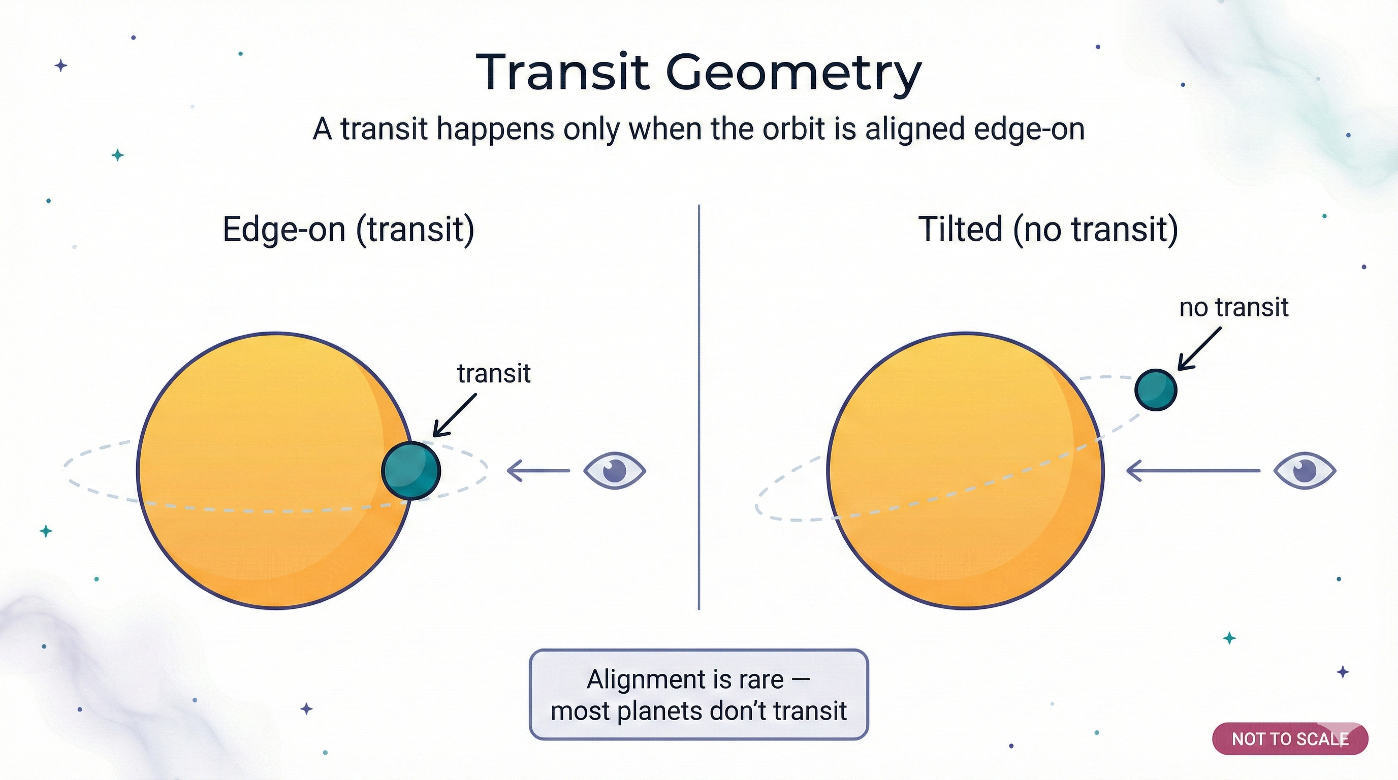
What to notice: transits require a lucky alignment — we only see a transit when the orbit is edge-on, so most planets do not transit from our viewpoint. (Credit: (A. Rosen/Gemini — schematic))
Remember from L4: Eclipses only happen when the Moon crosses the plane of Earth’s orbit (the ecliptic). Most months, the Moon passes above or below the Sun and no eclipse occurs.
The same geometry applies to exoplanet transits:
- We only see a transit if the planet’s orbit is edge-on to our line of sight
- Most exoplanets DON’T transit — their orbits are tilted relative to us
- Transit probability: roughly \(R_{\text{star}}/a\) (larger star or closer planet \(\rightarrow\) more likely)
This means transit surveys miss most planets, but the ones they find are gold: we know exactly how the orbit is tilted (edge-on)!
Selection effect: Because transit probability scales as \(R_*/a\), transit surveys are biased toward close-in planets with short orbital periods. Hot Jupiters were the first transiting exoplanets discovered for exactly this reason — they’re big and close to their stars.
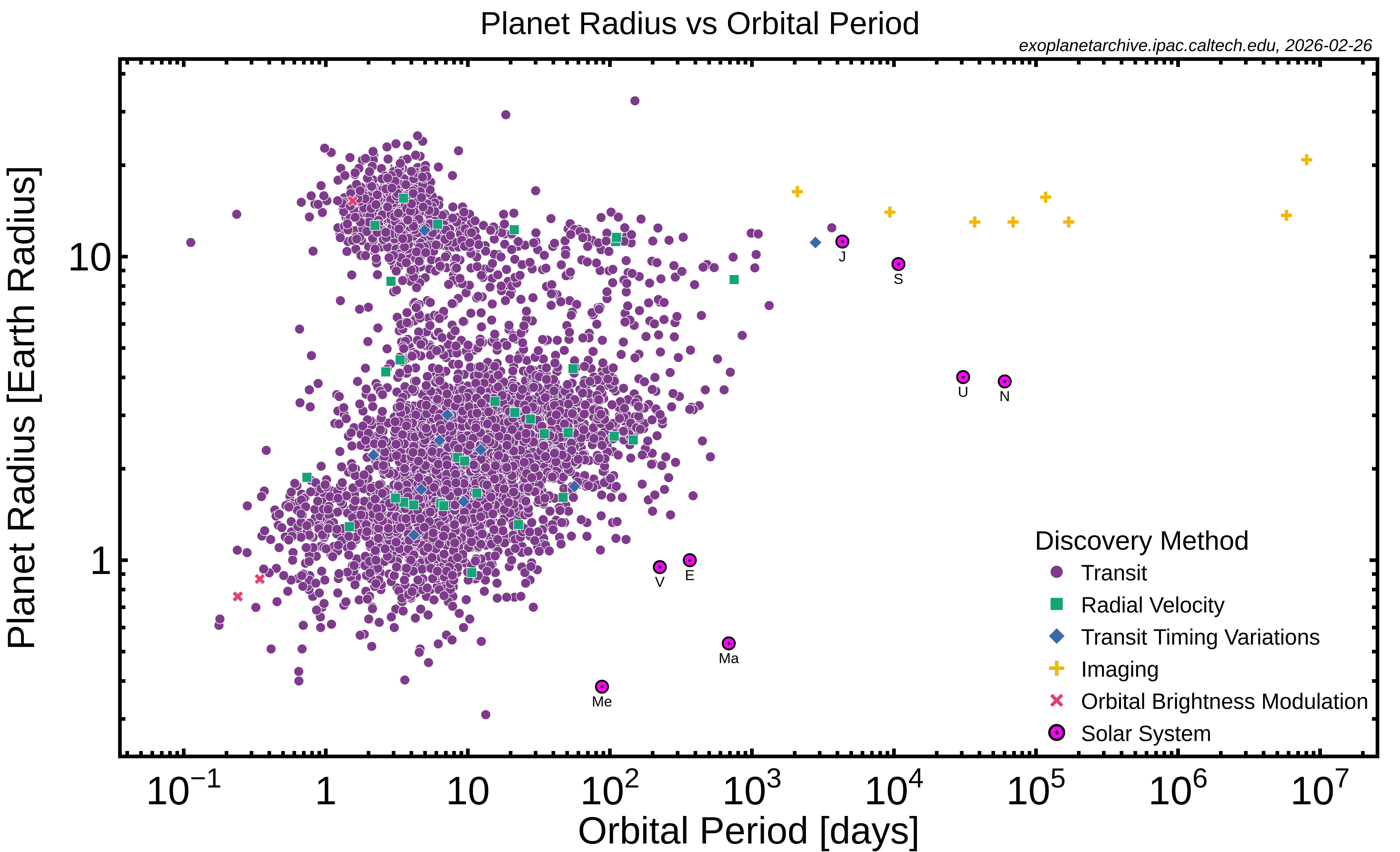
What to notice: detected planets cluster at short periods because transits are more likely and repeat faster there. This map is powerful, but it is detection-biased rather than a complete census. (Credit: NASA Exoplanet Archive (exported 2026-02-26))
This population view makes the selection effect concrete: we have many detections at short periods because those systems transit more often and are easier to confirm in finite observing campaigns.
The Transit Light Curve
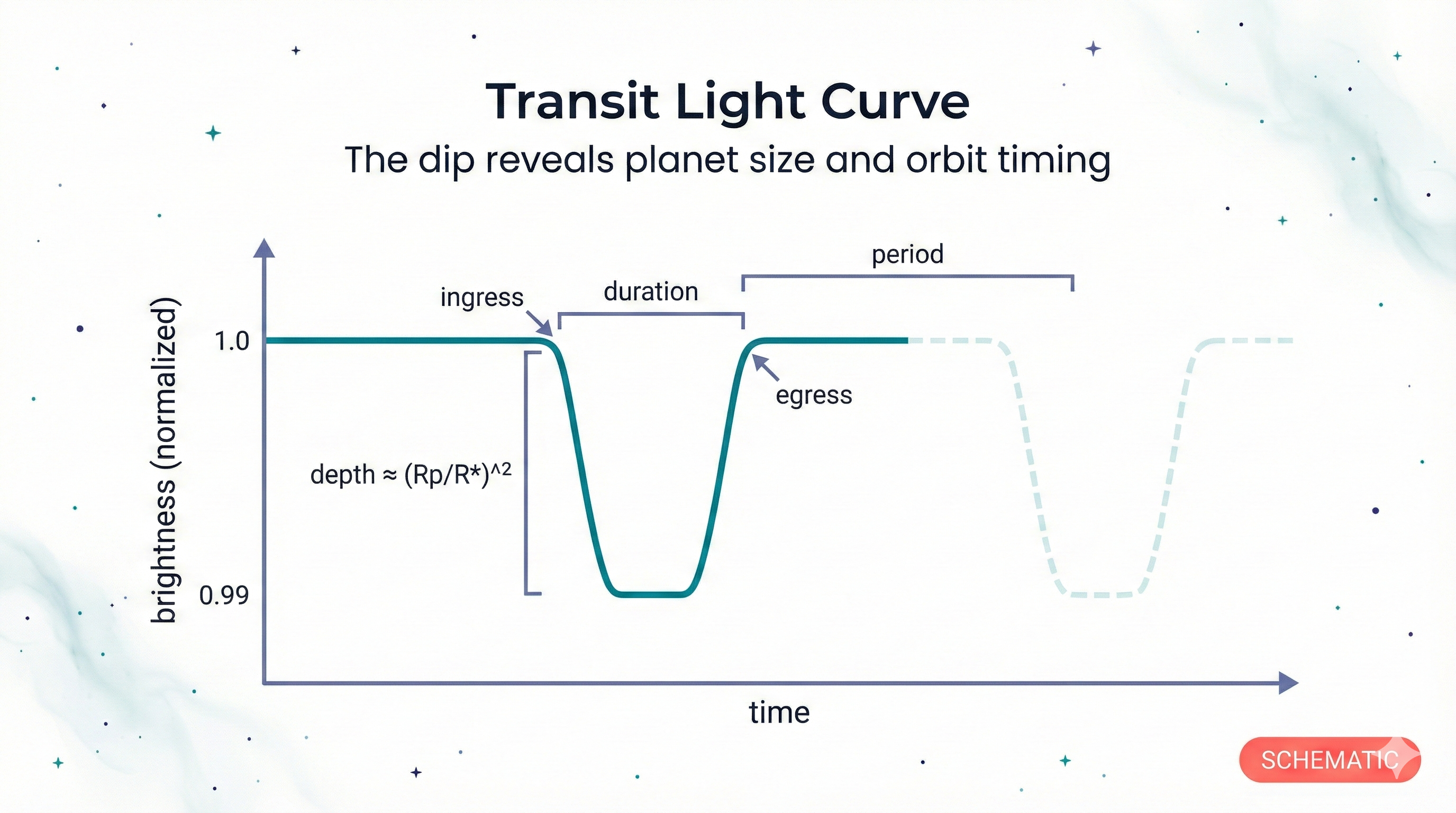
What to notice: the dip depth sets planet size (≈ (Rp/R*)²) and the timing between dips sets the orbital period. (Credit: (A. Rosen/Gemini — schematic))
What We Learn from Transits
| Observable | What It Tells Us |
|---|---|
| Transit depth | Planet radius: depth \(\approx\) \((R_p/R_*)^2\) |
| Transit duration | Orbital distance (combined with period, stellar mass, and transit geometry) |
| Orbital period | Time between transits |
| Orbital inclination | Must be nearly edge-on (~\(90^{\circ}\)) to transit |
Worked Example: How Big Is the Planet?
Problem: A star’s brightness drops by 1% during transit. If the star is Sun-sized (\(R_* = R_\odot\)), how big is the planet?
Solution:
The transit depth is the fraction of starlight blocked:
\[ \text{depth} = \left(\frac{R_p}{R_*}\right)^2 = 0.01 \]
Solving for planet radius:
\[ \frac{R_p}{R_*} = \sqrt{0.01} = 0.1 \]
\[ R_p = 0.1 \times R_\odot = 0.1 \times 696{,}000 \text{ km} = 69{,}600 \text{ km} \]
This is almost exactly Jupiter’s radius (71,500 km). A 1% dip indicates a Jupiter-sized planet!
Observable: A star’s brightness dips by 1% every 3.5 days, lasting a few hours each time. (Brightness + Timing)
Model: Transit depth \(= (R_p/R_*)^2\). The dip fraction equals the area ratio of planet to star.
Inference: \(R_p = 0.1 \, R_* \approx 69{,}600\) km — a Jupiter-sized planet. Same pattern as always: measurement \(\rightarrow\) physics \(\rightarrow\) knowledge.
An Earth-sized planet transiting a Sun-sized star would produce what transit depth? (Earth’s radius is ~1% of the Sun’s radius)
- 1%
- 0.1%
- 0.01%
- 0.001%
C) 0.01%. Transit depth = \((R_p/R_*)^2 = (0.01)^2 = 0.0001 = 0.01\%\). Earth-sized planets are MUCH harder to detect than Jupiter-sized planets! The Kepler and TESS missions had to achieve incredible photometric precision to find them.
Combining Methods — Density and Composition
The Power of Combining RV + Transit
When a planet both transits and shows radial velocity variations, we hit the jackpot:
| Method | What It Gives Us |
|---|---|
| Transit | Planet radius (\(R_p\)) |
| Radial velocity | Planet mass (\(M_p\)) — and since it transits, \(\sin i \approx 1\), so we get TRUE mass |
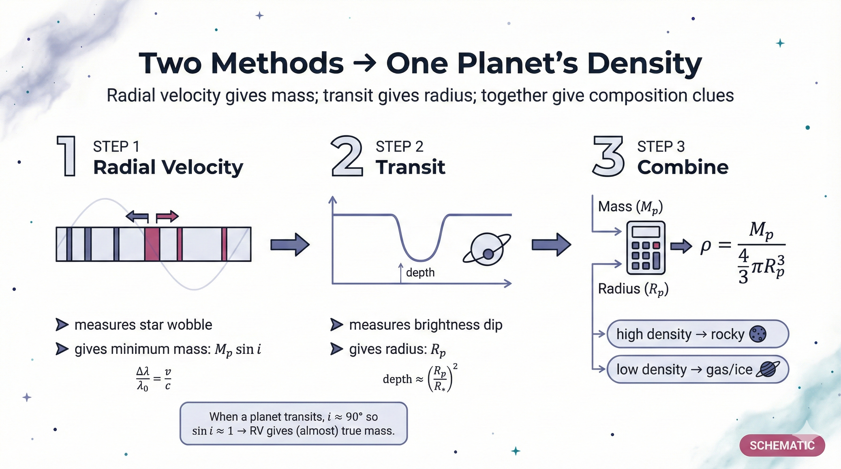
What to notice: radial velocity gives planet mass (or minimum mass), transit gives radius; together they give density — a first clue to rocky vs gas/ice composition. (Credit: (A. Rosen/Gemini — schematic))
With both mass and radius:
\[ \text{Density} = \frac{M_p}{\frac{4}{3}\pi R_p^3} \]
What Density Tells Us
| Density | Composition | Example |
|---|---|---|
| ~5.5 \(g/cm^{3}\) | Rocky (iron + silicate) | Earth |
| ~1.3 \(g/cm^{3}\) | Gas giant (H/He) | Jupiter |
| ~2-3 \(g/cm^{3}\) | Water world? Mini-Neptune? | Some super-Earths |
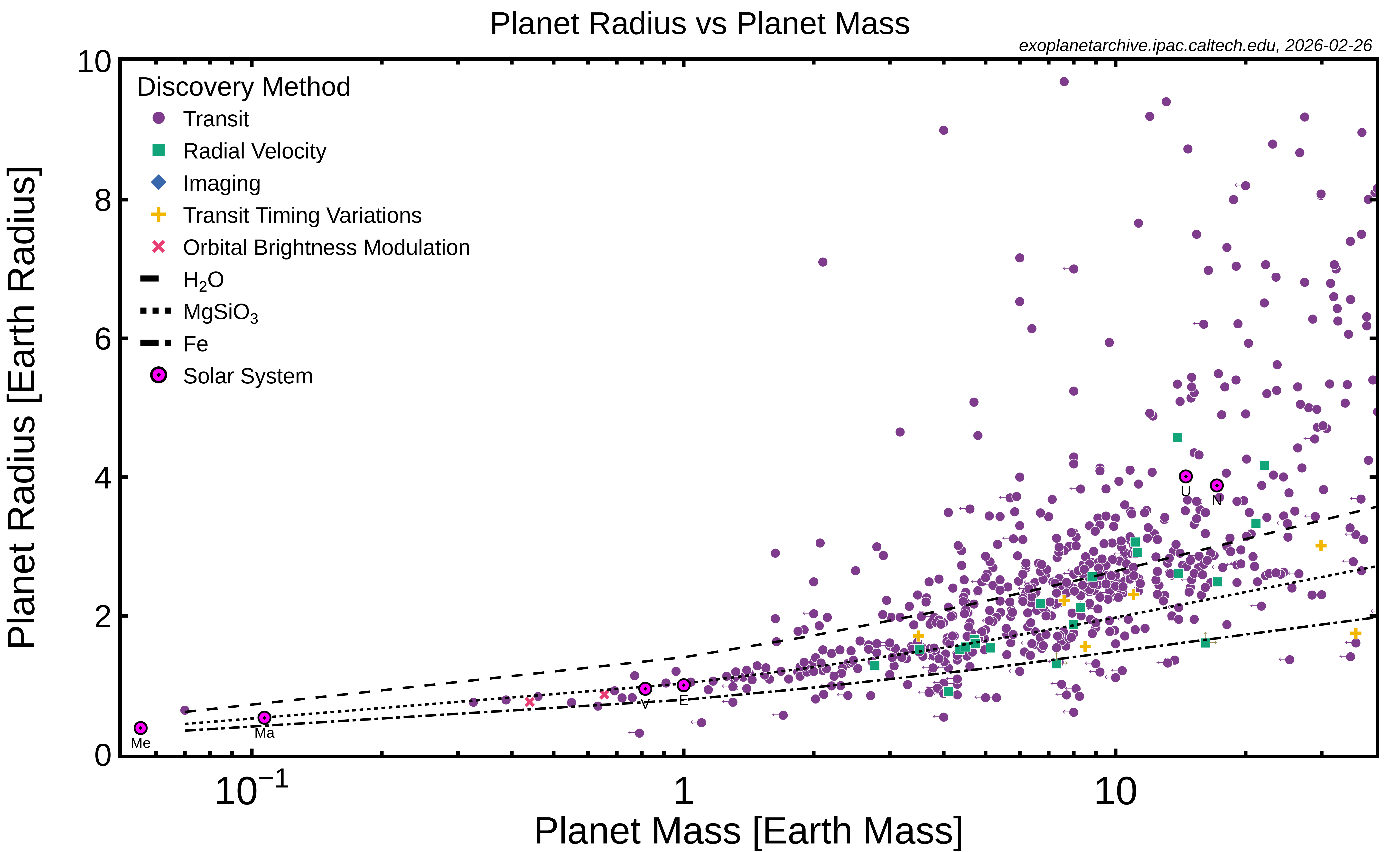
What to notice: mass plus radius constrains composition. Reference curves for iron, silicate rock, and water show why radius alone cannot uniquely identify what a planet is made of. (Credit: NASA Exoplanet Archive (exported 2026-02-26))
Intermediate densities (2–4 \(g/cm^{3})\) can be degenerate: different mixtures of rock, water, and gas can produce the same bulk density. Density is a strong clue to composition, but not a complete answer — additional constraints (atmospheric spectra, formation models) help break the degeneracy.
Observable: Radial velocity gives \(M_p = 5 \, M_\oplus\); transit gives \(R_p = 1.5 \, R_\oplus\). (Wavelength + Brightness + Timing)
Model: Density \(= M /V = M /(\tfrac{4}{3}\pi R^3)\). Scale to Earth: \(\rho \approx 5.5 \times (5 /1.5^3) \approx 8.1\) g/cm\(^3\).
Inference: Denser than Earth (5.5 g/cm\(^3\)) and far denser than Jupiter (1.3 g/cm\(^3\)) — a rocky, likely iron-rich super-Earth. Composition diagnosed from two measurements and one formula.
Density distinguishes rocky planets (potential for habitability) from gas/ice worlds (probably not habitable at the surface).
You discover a transiting planet with mass \(= 5 \, M_\oplus\) and radius \(= 1.5 \, R_\oplus\). Is it likely rocky or gaseous?
- Gaseous — any planet above \(1 \, M_\oplus\) must be a gas giant
- Rocky — its density is higher than Earth’s
- Impossible to tell without atmospheric spectra
- It must be a water world
B) Rocky. Density \(\approx 5.5 \times (5 /1.5^3) \approx 8.1\) g/cm\(^3\) — denser than Earth (5.5 g/cm\(^3\)) and far denser than Jupiter (1.3 g/cm\(^3\)). This planet is almost certainly rocky and iron-rich. Gas giants have densities \(\lesssim 2\) g/cm\(^3\); this planet is well above that threshold.
The Habitable Zone
The Goldilocks Zone
The habitable zone is the range of distances from a star where liquid water could exist on a planet’s surface — not too hot (water boils), not too cold (water freezes).
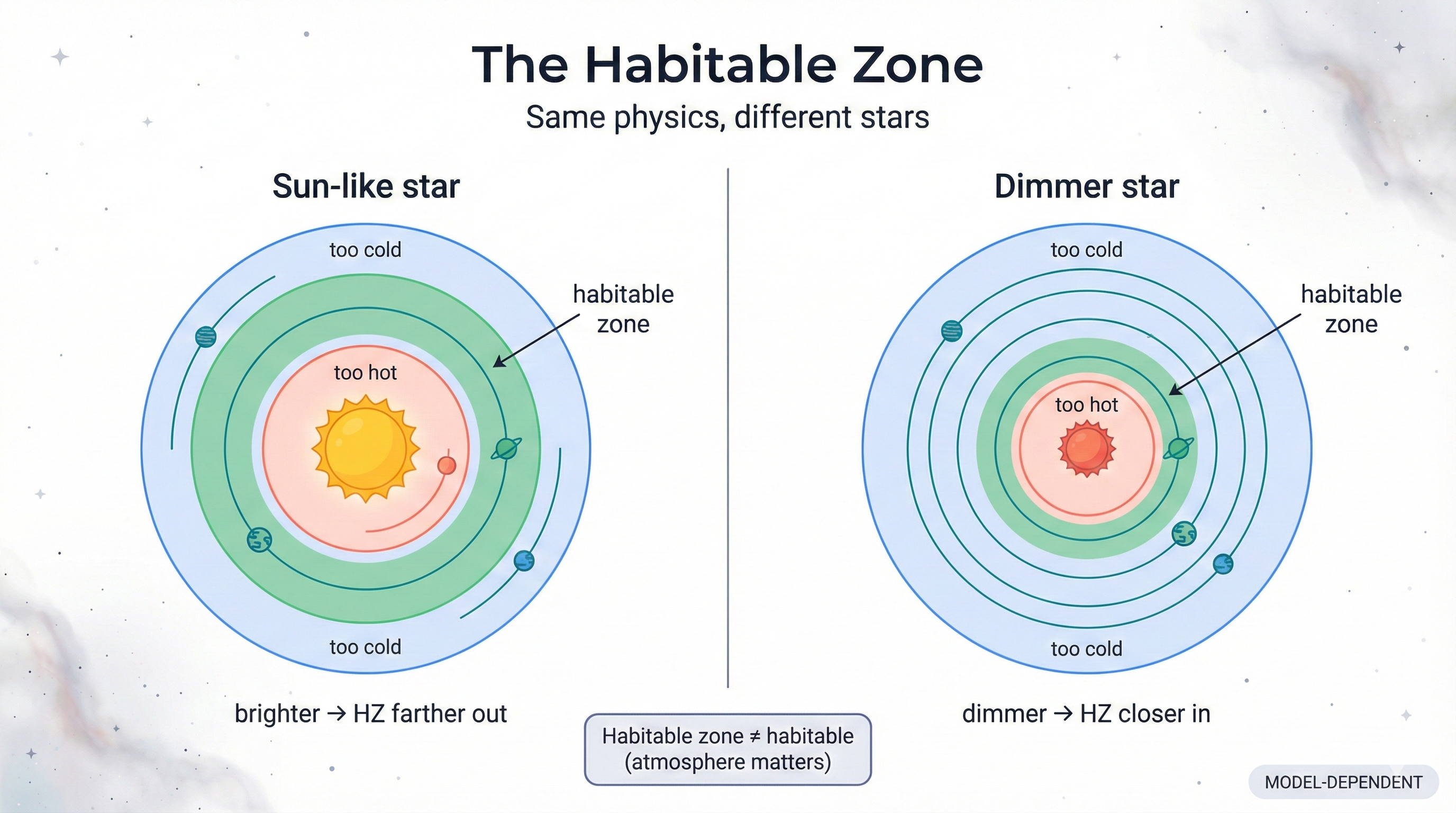
What to notice: habitable zone distance depends on stellar luminosity — brighter stars push the zone outward, dimmer stars pull it inward — and the zone is not a guarantee of habitability. (Credit: (A. Rosen/Gemini — schematic)) 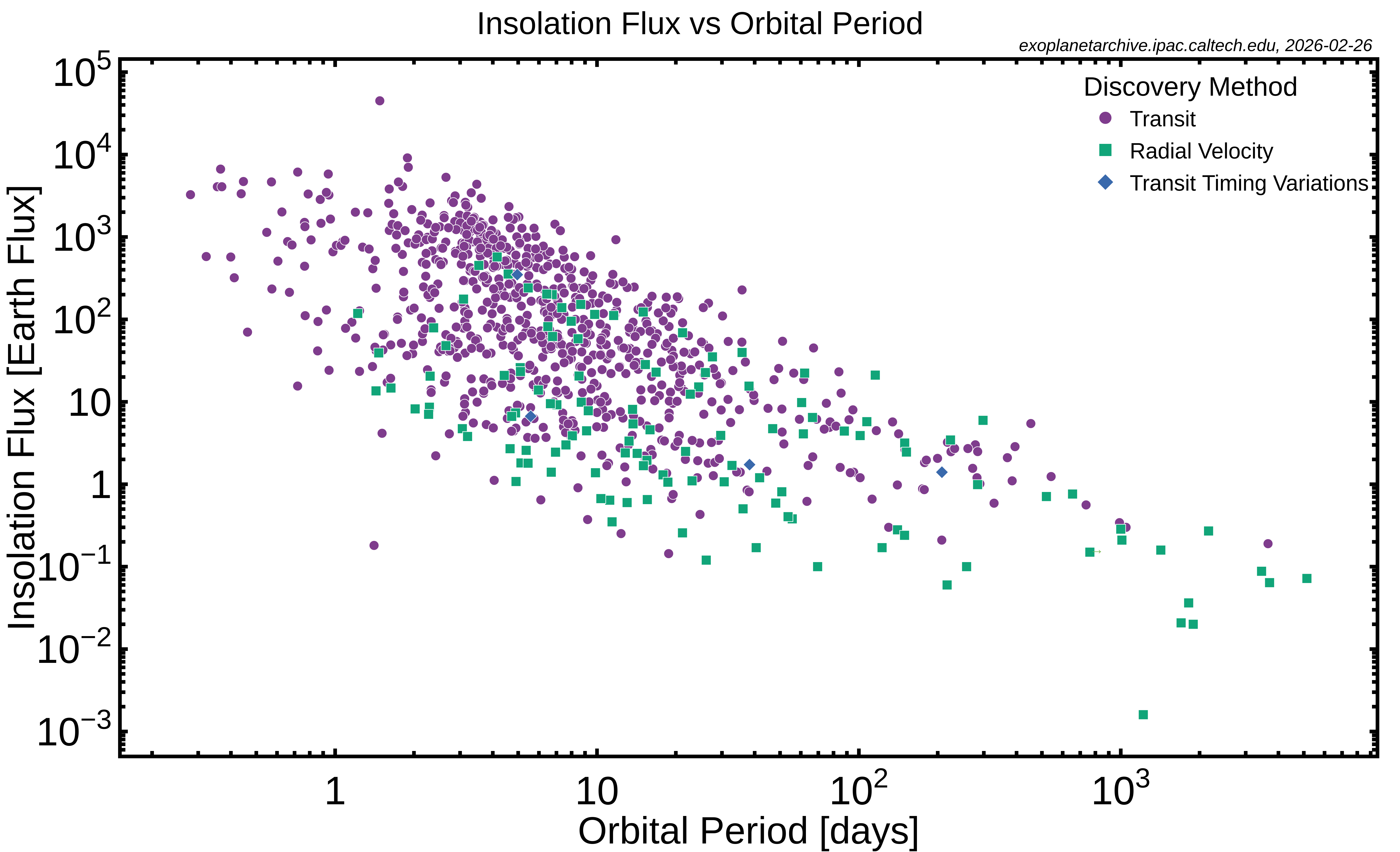
What to notice: average stellar flux drops with orbital period, but planets at the same period can sit at very different fluxes because host stars have different luminosities. (Credit: NASA Exoplanet Archive (exported 2026-02-26))
Notice how the points slope downward overall: longer-period planets usually receive less flux. But the large vertical spread at fixed period reminds us that host-star luminosity matters just as much as orbital distance.
What Determines the Habitable Zone?
The habitable zone depends on:
Stellar luminosity: More luminous star \(\rightarrow\) HZ is farther out (Stefan-Boltzmann callback!)
Atmospheric greenhouse effect: Strong greenhouse \(\rightarrow\) HZ extends farther out
Planetary albedo: More reflective \(\rightarrow\) needs to be closer to absorb enough heat
For the Sun (approximate, model-dependent):
- Inner edge: ~0.95–0.99 AU (Venus is just inside — but runaway greenhouse happened)
- Outer edge: ~1.4–1.7 AU (Mars is near the edge — and had liquid water with a thicker early atmosphere)
These boundaries depend on assumptions about atmospheric composition, cloud feedbacks, and planetary rotation. Different climate models give different estimates — the numbers above span “conservative” to “optimistic” 1-D models.
Habitable Zone \(\ne\) Habitable
Being in the habitable zone doesn’t guarantee a planet is habitable!
Venus is inside the inner edge (0.72 AU, closer to the Sun than the HZ) and is a 735 K hellscape. Mars is near the outer edge and is a frozen desert.
Habitability depends on:
- Having an atmosphere (and keeping it)
- The right greenhouse effect
- Liquid water on the surface
- Perhaps: magnetic field, plate tectonics, and more
The habitable zone is a starting point, not a guarantee.
Spot the assumption: The HZ assumes life needs liquid water on the surface. But Jupiter’s moon Europa and Saturn’s moon Enceladus have subsurface oceans far outside the HZ, heated by tidal forces rather than sunlight. If life can thrive in subsurface oceans, “habitability” extends well beyond the traditional zone.
If a star is \(4\times\) as luminous as the Sun, how does its habitable zone compare?
- Same location as the Sun’s
- Closer to the star
- Farther from the star
- There is no habitable zone
C) Farther from the star. A more luminous star delivers more energy, so planets at Earth’s distance would be too hot. The habitable zone moves outward by a factor of \(\sqrt{4} = 2\). If the Sun’s HZ is at ~1 AU, this star’s HZ would be at ~2 AU.
Looking for Signs of Life
Finding a planet in the habitable zone is just the beginning. The next question is: does it show signs of life? That’s the domain of biosignatures — atmospheric gases or surface features that would be difficult to explain without biology.
What Are Biosignatures?
Life doesn’t just exist — it transforms its environment. Earth’s atmosphere is wildly out of chemical equilibrium: oxygen (\(\text{O}_2\)) and methane (\(\text{CH}_4\)) coexist, even though they react with each other and should disappear within millions of years. The only reason both persist is that life continuously replenishes them — photosynthesis produces \(\text{O}_2\), and methanogenic microbes produce \(\text{CH}_4\).
Chemical disequilibrium: When reactive gases coexist in an atmosphere despite reacting with each other, something must be replenishing them. On Earth, that something is life.
If we found \(\text{O}_2\) and \(\text{CH}_4\) together in an exoplanet’s atmosphere, that chemical disequilibrium would be strong (though not conclusive) evidence for biology. Other potential biosignatures include ozone (\(\text{O}_3\), produced from \(\text{O}_2\)) and certain surface reflectance signatures from pigments like chlorophyll.
How Do We Detect Exoplanet Atmospheres?
Remember L9? Every molecule has a unique spectral fingerprint — specific wavelengths where it absorbs light. We used this to identify elements in stellar atmospheres. Now the same technique lets us read exoplanet atmospheres.
The key technique is transmission spectroscopy: during a transit, some starlight passes through the planet’s atmosphere before reaching us. Different wavelengths are absorbed by different atmospheric molecules, imprinting absorption lines onto the star’s spectrum. By comparing the spectrum during transit to the spectrum outside transit, we can identify which gases are present.
JWST: A New Era
The James Webb Space Telescope (launched December 2021) has the sensitivity to detect atmospheric molecules in exoplanet transit spectra. In 2022, JWST detected carbon dioxide (\(\text{CO}_2\)) in the atmosphere of WASP-39b — the first unambiguous detection of \(\text{CO}_2\) in an exoplanet atmosphere. JWST has since detected \(\text{SO}_2\) (sulfur dioxide, produced by photochemistry) in the same planet, demonstrating that we can study atmospheric chemistry, not just composition.
These are giant, hot planets — not habitable — but they prove the technique works. Applying the same method to smaller, cooler, rocky planets in habitable zones is the next frontier.
Why would detecting \(\text{O}_2\) and \(\text{CH}_4\) together in an exoplanet’s atmosphere be significant?
- Both gases are common in all planetary atmospheres
- They react with each other and shouldn’t coexist without something replenishing them
- They prove the planet has liquid water
- They indicate volcanic activity
B) They react with each other and shouldn’t coexist. Oxygen and methane are chemically reactive — left alone, they’d combine and disappear within millions of years. Finding both together means something is continuously producing them. On Earth, that something is life (photosynthesis makes \(\text{O}_2\); methanogens make \(\text{CH}_4\)). This chemical disequilibrium is one of the strongest potential biosignatures we could detect remotely.
We’ve now built a complete chain: find planets (transit + RV) \(\to\) measure their properties (radius, mass, density) \(\to\) identify habitable-zone candidates \(\to\) search for biosignatures in their atmospheres.
In L13, we’ll zoom out and ask the biggest question of all: How many civilizations might exist in the Galaxy? The Drake Equation takes everything we’ve learned — star formation, planet frequency, habitability — and tries to estimate the answer. It’s the ultimate application of the Observable \(\to\) Model \(\to\) Inference pattern to a question we can’t yet answer definitively.
Planetary Climates:
- Equilibrium temperature depends on distance from Sun and albedo
- Greenhouse effect: Atmosphere absorbs IR \(\rightarrow\) surface warms above equilibrium
- Venus: Runaway greenhouse \(\rightarrow\) 735 K hellscape
- Mars: Too little atmosphere \(\rightarrow\) 218 K frozen desert
- Earth: Moderate greenhouse, liquid water, life — adding \(\mathrm{CO_{2}}\) shifts the balance
Exoplanet Detection:
- Radial velocity: Star wobble \(\rightarrow\) minimum planet mass
- Transit: Brightness dip \(\rightarrow\) planet radius (depth = \((R_p/R_*)^2\))
- Combined: Mass + radius \(\rightarrow\) density \(\rightarrow\) rocky vs. gaseous
- Habitable zone: Where liquid water could exist (depends on stellar luminosity)
- Biosignatures: Chemical disequilibrium (e.g., \(\text{O}_2\) + \(\text{CH}_4\)) as evidence for life; JWST can detect atmospheric molecules via transmission spectroscopy
Practice Problems
Solutions are available in the Lecture 12 Solutions.
Core (do these first)
1. Greenhouse Calculation: Earth’s equilibrium temperature is ~255 K, but its actual surface temperature is ~288 K. Calculate the greenhouse warming effect in Kelvin. Compare to Venus (\(T_{\text{eq}} \approx 230\) K, \(T_{\text{actual}} = 735\) K).
2. Transit Depth: A planet with radius \(2 \times\) Earth’s transits a Sun-like star. What is the transit depth? By what factor is this easier to detect than an Earth-sized planet?
3. Habitable Zone Scaling: A star has luminosity \(1/4\) that of the Sun. Where is its habitable zone compared to the Sun’s? (Hint: the habitable zone distance scales as \(\sqrt{L/L_\odot}\).)
4. Detection Methods: You detect a planet via both radial velocity (star wobbles at 100 m/s) and transit (1% depth). What two properties can you now calculate that you couldn’t with just one method?
5. Albedo and Equilibrium Temperature: Earth’s equilibrium temperature with its current Bond albedo (\(A = 0.30\)) is 255 K. If Earth’s albedo increased to 0.40 (e.g., more ice and cloud cover), what would the new equilibrium temperature be? Use the scaling \(T_{\text{eq}} \propto (1 - A)^{1/4}\).
6. Radial Velocity Detection: A Sun-like star shows a periodic radial velocity wobble of 50 m/s with a period of 4.2 days. Is the companion more likely a planet or a star? Compare to Jupiter’s effect on the Sun (~13 m/s, period 12 years). What does the short period suggest about the planet’s orbit?
Challenge
7. Habitable Zone Width: The Sun’s habitable zone extends from roughly 0.95 AU to 1.4 AU. A red dwarf star with luminosity \(L = 0.01\,L_\odot\) has its habitable zone scaled inward by \(\sqrt{L/L_\odot}\). Calculate the inner and outer edges. How does the width of this habitable zone compare to the Sun’s?
8. Biosignature Reasoning: Earth’s atmosphere contains both \(\mathrm{O_{2}}\) (produced by photosynthesis) and \(\mathrm{CH_{4}}\) (produced by biology and geology). These two gases react with each other and would disappear without continuous replenishment. Explain why detecting both \(\mathrm{O_{2}}\) and \(\mathrm{CH_{4}}\) in an exoplanet atmosphere would be more compelling evidence for life than detecting either one alone.
9. Venus’s History: Explain in your own words how Venus went from possibly habitable to its current state. Include the role of distance from the Sun, water vapor feedback, and \(\mathrm{CO_{2}}\) accumulation.
10. Density Interpretation: You discover a planet with the same mass as Neptune (\(1.02 \times 10^{26}\) kg) but the same radius as Earth (\(6.37 \times 10^6\) m). Calculate its average density and compare to Earth (5.5 \(g/cm^{3})\) and Neptune (1.6 \(g/cm^{3}).\) What might this planet be made of?
Glossary
- ★ Bond albedo
- The fraction of total incoming stellar energy reflected back to space by a planet, averaged over wavelength and direction. Energy balance uses absorbed fraction \((1-A)\), where \(A\) is Bond albedo.
- ★ Bulk density
- Average density of a planet, computed from mass and radius. \(\rho = M/(\tfrac{4}{3}\pi R^3)\); used to infer broad composition classes (rocky vs gas-rich).
- ★ Chemical disequilibrium
- A state where reactive atmospheric gases coexist away from thermodynamic equilibrium and require continuous replenishment. Coexisting O\(_2\) and CH\(_4\) is a canonical biosignature candidate.
- ◇ Effective emission level
- The characteristic altitude in an atmosphere from which most thermal radiation escapes to space. If greenhouse opacity increases, this level shifts higher and colder, so the surface must warm to restore balance.
- ★ Equilibrium temperature
- The temperature a planet would have if absorbed sunlight balanced emitted thermal radiation, ignoring atmospheric greenhouse warming. For a planet at distance d with albedo A: \(T_{\mathrm{eq}} \propto [(1-A)/d^2]^{1/4}\).
- ★ Exoplanet
- A planet orbiting a star other than the Sun. Over 5,000 confirmed as of 2024; many are unlike anything in our solar system.
- ◇ Exoplanet atmosphere
- The gaseous envelope around an exoplanet, inferred remotely through spectra and transit/eclipse observations. Atmospheric composition constrains climate, chemistry, and possible biosignatures.
- ★ Greenhouse effect
- The warming of a planet's surface when atmospheric gases absorb and re-emit infrared radiation. CO₂, H₂O, CH₄ are key greenhouse gases; Venus is an extreme example.
- ★ Greenhouse gas
- A gas that absorbs and re-emits infrared radiation, tending to warm a planet's surface. Key examples include H\(_2\)O, CO\(_2\), CH\(_4\), and N\(_2\)O.
- ★ Habitable zone
- The range of orbital distances from a star where liquid water could exist on a planet's surface. Also called the 'Goldilocks zone'; depends on stellar luminosity.
- ◇ Hot Jupiter
- A gas giant exoplanet orbiting very close to its star (< 0.1 AU), with orbital periods of days. Easiest to detect but puzzling—gas giants should form far from their stars.
- ◇ Insolation flux
- The stellar energy flux received by a planet at its orbit. Often reported in Earth-flux units to compare irradiation levels across exoplanets.
- ★ Minimum mass ($M_p\sin i$)
- The lower bound on planet mass measured by radial velocity when inclination is unknown. If a planet also transits, then \(\sin i \approx 1\) and radial velocity gives near-true mass.
- ★ Orbital inclination (i)
- The tilt of an orbit relative to the observer's line of sight. Transits require nearly edge-on geometry (\(i \approx 90^{\circ}\)).
- ★ Planetary atmosphere
- A layer of gases surrounding a planet that can absorb, emit, and transport energy. Atmospheric thickness and composition control greenhouse warming strength.
- ★ Planetary climate
- The long-term thermal and atmospheric state of a planet, set by energy input, energy loss, and atmospheric/oceanic processes. In this lecture: sunlight in, infrared out, plus greenhouse feedbacks.
- ★ Planetary habitability
- The potential of a planet to support life, commonly evaluated first by the possibility of stable liquid water. Habitable zone membership is a starting screen, not a guarantee of habitability.
- ★ Radial velocity method
- Detecting exoplanets by measuring the Doppler shift caused by the star's wobble around the system's center of mass. Gives minimum planet mass; most effective for massive planets close to their stars.
- ◇ Runaway greenhouse
- A feedback loop where rising temperatures evaporate more water, which traps more heat, leading to extreme warming. May explain Venus's current state; a cautionary tale for Earth's climate.
- ★ Transit depth
- The fractional drop in stellar brightness during a transit. To first order, depth \(\approx (R_p/R_*)^2\), so depth constrains planet radius.
- ★ Transit method
- Detecting exoplanets by measuring the tiny dimming when a planet passes in front of its star. Gives planet size; requires edge-on orbital alignment.
- ◇ Transit probability
- The chance that an exoplanet system is aligned so a transit is visible from Earth. Approximately scales as \(R_*/a\) for circular orbits, so close-in planets transit more often.
- ★ Transmission spectroscopy
- Measuring wavelength-dependent starlight filtering through a transiting planet's atmosphere to identify atmospheric gases. Compare in-transit and out-of-transit spectra to isolate atmospheric absorption features.