Motion Revealed — Doppler Effect and the Astronomer’s Toolkit
Lecture 10 Reading Companion
The Big Idea
In L9, we learned that spectral lines are chemical fingerprints — each element absorbs and emits at specific wavelengths. But what happens when those fingerprints shift? A shifted spectral line means the source is moving. The Doppler effect lets us measure velocities across cosmic distances — revealing orbiting exoplanets, spinning galaxies, and the invisible dark matter that holds them together. And telescopes are the eyes that collect this light, letting us decode the cosmos.
This reading covers the Doppler effect and telescopes — completing the astronomer’s toolkit.
Structure:
- Part 1: The Doppler effect — motion from wavelength shifts
- Part 2: Telescopes — collecting the light
Musts for today (~40-50 min):
- The Doppler formula and what each term means
- Radial vs. transverse velocity (crucial distinction!)
- Exoplanet detection via stellar wobbles
- Dark matter evidence from galaxy rotation curves
- Light-gathering power and resolution basics
Non-negotiable: Stop at every Check Yourself question — don’t just read past them!
This lecture completes Module 1. You now have all the tools:
- Motion reveals mass (L5-L6)
- Light reveals temperature (L7-L8)
- Spectral lines reveal composition (L9)
- Doppler reveals motion; telescopes collect the light (L10)
In Module 2, we apply these tools to stars.
If you only remember three things:
Doppler effect: \(\Delta\lambda/\lambda_0 = v/c\). Blueshift = approaching; redshift = receding. Only measures radial (line-of-sight) velocity.
Motion reveals mass (again!): Stellar wobbles reveal exoplanets. Galaxy rotation curves reveal dark matter. Same principle as L5-L6, now applied with spectroscopy.
Telescopes: Bigger mirrors collect more light (\(\propto D^2\)) and see finer detail (resolution \(\propto \lambda/D\)). Space telescopes access wavelengths blocked by atmosphere.
Now for the details…
The Fingerprints Move
In L9, we learned to read chemical fingerprints in starlight. Hydrogen always absorbs at 656.28 nm \((H\alpha),\) sodium at 589.0 nm — these patterns are as reliable as barcodes.
But astronomers noticed something strange. When they observed distant stars and galaxies, the fingerprints weren’t always at the expected wavelengths. Sometimes the hydrogen line appeared at 656.50 nm. Sometimes at 656.10 nm. The pattern was shifted.
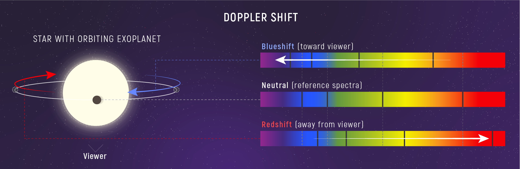
What to notice: Doppler shift moves spectral lines—toward blue for motion toward us and toward red for motion away—so spectra can measure motion. (Credit: Illustration: NASA, ESA, CSA)
The culprit? Motion. Just as an ambulance siren sounds higher-pitched when approaching and lower when receding, light waves get compressed or stretched depending on whether the source moves toward or away from us. This is the Doppler effect — and it’s one of astronomy’s most powerful tools.
Today we’ll learn how to extract velocities from wavelength shifts. We’ll discover exoplanets through stellar wobbles, and we’ll uncover evidence for invisible dark matter in galaxy rotation curves. And we’ll explore the telescopes — the astronomer’s eyes — that collect the light carrying all this information.
In Lecture 9, we discovered how composition is written in light:
- Kirchhoff’s Laws: continuous, emission, and absorption spectra
- Quantized energy levels \(\rightarrow\) discrete spectral lines
- Each element has a unique fingerprint
- OBAFGKM classification orders stars by temperature
Now we ask: what happens when those fingerprints shift?
Part 1: The Doppler Effect
Gravity Makes Everything Move
In Lectures 5 and 6, we learned that gravity is a long-range force — it reaches across the cosmos, pulling on everything with mass. This means everything in the universe is in motion:
- Planets orbit stars
- Stars orbit galaxy centers
- Galaxies fall toward each other in clusters
- Even “stationary” stars are moving at tens of km/s through space
All this motion leaves a signature in light: the Doppler effect. By measuring wavelength shifts, we measure velocity — and from velocity, we can infer mass, detect invisible companions, and reveal the hidden structure of the universe.
This is the ultimate payoff of the throughline we’ve been building:
Motion reveals mass (L5-L6) + Light carries information (L7-L9) = Spectral line shifts reveal motion (L10)
The Doppler Effect
The Familiar Version (Sound)
You’ve heard the Doppler effect even if you didn’t know its name. An ambulance siren sounds higher-pitched as it approaches and lower-pitched as it recedes. A race car’s engine note drops as it zooms past. What’s happening?
Sound waves from an approaching source get compressed — the waves pile up, making the wavelength shorter and the frequency higher (higher pitch). Sound waves from a receding source get stretched — the waves spread out, making the wavelength longer and the frequency lower (lower pitch).
For Light: Wavelength Shifts
Light behaves the same way:
- Source moving toward you \(\rightarrow\) wavelengths compressed \(\rightarrow\) shifted toward shorter wavelengths
- Source moving away from you \(\rightarrow\) wavelengths stretched \(\rightarrow\) shifted toward longer wavelengths
\[ \frac{\Delta\lambda}{\lambda_0} = \frac{v}{c} \]
where:
- \(\lambda_0\) = the rest wavelength (measured in the lab, with no relative motion)
- \(\Delta\lambda = \lambda_{observed} - \lambda_0\) = the wavelength shift
- \(v\) = the object’s radial velocity (along the line of sight)
- \(c = 3 \times 10^5\) km/s (speed of light)
Positive \(\Delta\lambda\) (wavelength increased) \(\rightarrow\) redshift \(\rightarrow\) moving away
Negative \(\Delta\lambda\) (wavelength decreased) \(\rightarrow\) blueshift \(\rightarrow\) moving toward
Rest wavelength (\(\lambda_0\)): The wavelength of a spectral line measured in the laboratory, with source and observer at rest relative to each other.
Radial velocity: The component of velocity along the line of sight — toward or away from the observer.
Redshift: Shift to longer wavelengths (source receding).
Blueshift: Shift to shorter wavelengths (source approaching).
This short video walks through the Doppler effect for both sound and light — a helpful complement to the reading above.
What Do These Symbols Mean?
Rest Wavelength: The Reference Point
Students often ask: “Rest wavelength relative to what?”
The answer: The rest wavelength (\(\lambda_0\)) is the wavelength a spectral line has when the source and observer are not moving relative to each other.
In practice: We measure rest wavelengths in the laboratory. We take a tube of hydrogen gas, excite it with electricity, and precisely measure the wavelengths of the emission lines. These laboratory values become our reference:
- Hydrogen-alpha \((H\alpha):\) \(\lambda_0 = 656.28\) nm
- Hydrogen-beta \((H\beta):\) \(\lambda_0 = 486.13\) nm
- Sodium D lines: \(\lambda_0 = 589.0\) nm and 589.6 nm
When we observe a star and see \(H\alpha\) at 656.50 nm instead of 656.28 nm, we know the line has been redshifted by \(\Delta\lambda = +0.22\) nm. That shift tells us the star is moving away from us.
Key point: The rest wavelength is our reference standard. Without knowing \(\lambda_0\) precisely, we couldn’t detect or measure the shift.
Here’s a wrinkle: Earth itself moves! Over a year, our orbital motion around the Sun shifts spectral lines by up to \(\pm30\) km/s.
Astronomers correct for this by converting observed velocities to a “barycentric” frame — the center of mass of the solar system. This removes Earth’s orbital motion, leaving only the motion of the source relative to the solar system.
Without this correction, the same star would appear to shift back and forth over the course of a year — not because it’s moving, but because we are!
Radial vs. Transverse Motion
Only Line-of-Sight Motion Creates Doppler Shifts
Here’s a crucial distinction that trips up many students:

What to notice: Doppler shifts measure only line-of-sight (radial) velocity; purely sideways (transverse) motion produces no wavelength shift. (Credit: Illustration: A. Rosen (SVG))
The Doppler effect measures only the radial velocity — the component of motion along your line of sight:
- Radial motion: Toward or away from you \(\rightarrow\) Doppler shift detected
- Transverse motion: Across your field of view \(\rightarrow\) No Doppler shift
A star moving purely sideways shows zero Doppler shift, even if it’s moving very fast!
Radial velocity: The component of an object’s velocity along the line of sight — toward or away from the observer. This is what the Doppler effect measures.
Transverse velocity: The component of velocity perpendicular to the line of sight — motion across the sky. Detected through proper motion (position change over years), not Doppler.
Line of sight: The imaginary line from the observer to the object being observed.
Why This Matters
If a star is moving at 100 km/s but entirely across the sky (transverse), you’ll measure zero Doppler shift. To detect that motion, you’d need to watch the star’s position change over years — called “proper motion.”
In most cases, an object’s motion is at some angle, so it has both radial and transverse components. The Doppler effect only reveals the radial part.
A star is moving at 100 km/s exactly perpendicular to your line of sight (directly across the sky). Its Doppler shift is:
- Large redshift
- Large blueshift
- Zero
- Cannot be determined
C) Zero. The Doppler effect only measures radial velocity (along the line of sight). Motion purely across the sky (transverse) produces no wavelength shift. To detect transverse motion, you’d need to measure the star’s position change over time (proper motion).
Blueshift and Redshift — A Naming Clarification
The names “blueshift” and “redshift” come from visible light:
- Blue is at the short-wavelength end of the visible spectrum
- Red is at the long-wavelength end
But the Doppler effect applies to ALL electromagnetic radiation — radio waves, infrared, X-rays, gamma rays, everything!
When astronomers say a radio source is “redshifted,” they don’t mean it turned red. They mean its wavelengths are shifted toward longer values — shifted in the “red direction” even if the light isn’t visible.
The naming convention:
- Blueshift = shifted to shorter wavelengths (any part of spectrum)
- Redshift = shifted to longer wavelengths (any part of spectrum)
An X-ray that gets “redshifted” is still an X-ray — just at a longer wavelength than its rest value.
The Doppler effect explains redshifts from motion through space — a galaxy moving away from us has its light redshifted.
But in Module 3, you’ll learn about cosmological redshift, which is caused by the expansion of space itself. Distant galaxies are redshifted not because they’re flying away through space, but because space between us and them has stretched while the light was traveling.
For now: Focus on Doppler redshift (motion through space). We’ll tackle cosmological redshift when we study the expanding universe.
Key difference:
- Doppler: Object moving through space \(\rightarrow\) wavelength shifted
- Cosmological: Space itself expanding \(\rightarrow\) wavelength stretched
Both produce redshifts, but the physics is different!
Worked Example: Measuring Stellar Velocity
Problem: A star’s \(H\alpha\) absorption line is observed at 656.50 nm. The laboratory (rest) wavelength of \(H\alpha\) is 656.28 nm. Find the star’s radial velocity. Is it approaching or receding?
Solution:
Step 1: Calculate the wavelength shift \[ \Delta\lambda = \lambda_{observed} - \lambda_0 = 656.50 - 656.28 = +0.22 \text{ nm} \]
Step 2: Calculate the fractional shift \[ \frac{\Delta\lambda}{\lambda_0} = \frac{0.22}{656.28} = 3.35 \times 10^{-4} \]
Step 3: Apply the Doppler formula \[ v = c \times \frac{\Delta\lambda}{\lambda_0} = (3 \times 10^5 \text{ km/s}) \times (3.35 \times 10^{-4}) = 100 \text{ km/s} \]
Step 4: Interpret the sign \(\Delta\lambda > 0\) means the wavelength increased (redshift), so the star is moving away from us at about 100 km/s.
Observable: A star’s \(H\alpha\) line appears at 656.50 nm instead of the lab value 656.28 nm.
Model: Doppler shift: \(\Delta\lambda/\lambda_0 = v/c\). Positive shift = receding.
Inference: The star is moving away from us at ~100 km/s. This is typical for nearby stars — they’re all in motion relative to the Sun.
A star’s sodium D line (rest wavelength 589.0 nm) is observed at 588.8 nm. The star is:
- Moving toward us at ~100 km/s
- Moving away from us at ~100 km/s
- Moving toward us at ~1000 km/s
- Not moving
A) Moving toward us at ~100 km/s.
\(\Delta\lambda = 588.8 - 589.0 = -0.2\) nm (negative = blueshift = approaching)
\(v = c \times |\Delta\lambda|/\lambda_0 = (3 \times 10^5) \times (0.2/589.0) \approx 100\) km/s toward us.
🔭 Demo Exploration: Doppler Shift Spectrometer
This demo overlays a rest spectrum and an observed spectrum so you can see Doppler shifts directly and practice the sign convention.
Mission A (sign)
Predict before you slide: When \(v_r\) is positive, is the star approaching or receding?
Write your prediction here: _______________
Mission B (radial vs transverse)
Switch to transverse motion. What happens to the spectrum? Explain why in one sentence.
Mission C (compute)
Pick a line and use the readouts to compute \(v = c\,\Delta\lambda/\lambda_0\). Then check your computed \(v\) against the demo.
Exoplanet Detection: The Radial Velocity Method
The Conceptual Idea
Here’s a beautiful application of the Doppler effect: detecting planets around other stars.
By Newton’s Third Law, a planet doesn’t just orbit its star — the star also wobbles in response. The planet pulls on the star just as the star pulls on the planet. Both orbit their common center of mass.
This stellar wobble is tiny — the Sun moves only about 12 m/s due to Jupiter’s pull — but it’s detectable with precise Doppler measurements. As the star wobbles toward and away from us, its spectral lines shift back and forth. The periodic pattern reveals an orbiting planet.
Expand the “Radial velocity method” panel and enable the RV overlay. Watch the spectral line shift back and forth as the RV curve marker moves — this is the measurement that produces the curve.
This NASA animation shows how a planet’s gravitational tug makes its star wobble — and how that wobble produces a periodic Doppler signal.

What to notice: an orbiting planet makes its star wobble; the star’s back-and-forth line-of-sight motion produces a periodic Doppler signal. (Credit: Illustration: A. Rosen (SVG))
Quantitative Example: Detecting a Hot Jupiter
Problem: A star’s spectral lines shift back and forth with an amplitude of \(\Delta\lambda = \pm 1.2 \times 10^{-4}\) nm around the \(H\alpha\) rest wavelength of 656.28 nm. The shift completes one cycle every 4.2 days. What is the star’s wobble velocity? What does this tell us?
Solution:
Step 1: Calculate the velocity amplitude \[ \frac{\Delta\lambda}{\lambda_0} = \frac{1.2 \times 10^{-4}}{656.28} = 1.8 \times 10^{-7} \] \[ v = c \times \frac{\Delta\lambda}{\lambda_0} = (3 \times 10^5 \text{ km/s}) \times (1.8 \times 10^{-7}) = 0.056 \text{ km/s} = 56 \text{ m/s} \]
Step 2: Interpret
The star wobbles at \(\pm56\) m/s with a 4.2-day period. This is larger than the Sun’s ~12 m/s wobble from Jupiter (which has a 12-year period), but still tiny — about the speed of a fast jog!
A short period (4.2 days) means the planet orbits very close to the star. Combined with the velocity amplitude, we can estimate the planet is about half a Jupiter mass.
This is the signature of a “hot Jupiter” — a massive planet in a tight orbit. The first exoplanet around a Sun-like star, 51 Pegasi b, was discovered exactly this way in 1995 (with v \(\approx\) 56 m/s and P = 4.2 days)!
Detecting a 56 m/s wobble seems impossible — but astronomers don’t measure one line at that precision. Instead, they track the centroids of many spectral lines simultaneously, gaining statistical power. Modern spectrographs like HARPS are kept in vacuum, stabilized to hundredths of a degree, and calibrated with thorium-argon lamps or laser frequency combs.
The result: velocity precision far better than the width of a single spectral resolution element. The 2019 Nobel Prize in Physics recognized Mayor & Queloz for their discovery of 51 Pegasi b using this approach.
The Information Payoff
From Doppler measurements alone, we can determine:
- Orbital period \(\rightarrow\) from the periodicity of the velocity curve
- Minimum planet mass \(\rightarrow\) from the velocity amplitude (minimum because we may not see the orbit edge-on)
- Orbital eccentricity \(\rightarrow\) from the shape of the velocity curve
Combined with transit observations (when a planet crosses in front of its star), we can get the planet’s true mass and size.
The radial velocity method detects exoplanets by measuring:
- The planet’s light directly
- The star’s periodic Doppler shift due to its wobble
- The planet blocking starlight during transit
- Gravitational lensing by the planet
B) The star’s periodic Doppler shift due to its wobble.
The planet’s gravity causes the star to move in a small orbit around the center of mass. This motion creates periodic Doppler shifts that we can measure. The planet itself is far too faint to see directly in most cases.
Dark Matter: When Orbits Don’t Add Up
The Galaxy Rotation Puzzle
In the 1970s, astronomer Vera Rubin used the Doppler effect to measure how fast stars orbit within spiral galaxies. She expected to find that stars far from the galaxy center orbit more slowly — just as outer planets in our solar system orbit more slowly than inner ones (Kepler’s Third Law).

What to notice: in the Solar System, orbital speed decreases with distance, following a Keplerian decline. (Credit: cococubed.com)
What she found was shocking: stars at the edges of galaxies move just as fast as stars near the center.
What to notice: galaxy rotation curves stay flat at large radii — visible matter alone would predict a decline, so extra mass is implied. (Credit: Figure: CoCoCubed (SVG))
Why This Is Strange
By Newton’s gravity and Kepler’s Laws, the orbital velocity should depend on the mass inside the orbit:
\[ v_{orbit} = \sqrt{\frac{GM_{interior}}{r}} \]
If most of a galaxy’s mass is concentrated in the bright central region, then at large distances, \(M_{interior}\) should be roughly constant, and \(v_{orbit}\) should decrease as \(1/\sqrt{r}\).
But the velocity stays flat. This means \(M_{interior}\) must keep increasing with distance — there’s more mass out there than we can see!
The Dark Matter Hypothesis
The leading explanation: there’s far more matter in galaxies than the visible stars, gas, and dust. This unseen matter doesn’t emit or absorb light (hence “dark”), but it has gravity.
We call it dark matter. It forms a huge, invisible halo surrounding galaxies, providing the extra gravitational pull that keeps outer stars orbiting so fast.
Dark matter: Invisible matter that doesn’t emit, absorb, or reflect light, but has gravitational effects. Makes up ~27% of the universe’s mass-energy — about \(5\times\) more than ordinary matter.
The Throughline: Motion Reveals Mass (Even Invisible Mass)
This is the ultimate payoff of L5-L6: motion reveals mass. Vera Rubin watched how stars move and discovered that most of a galaxy’s mass is invisible.
We’ve never directly detected a dark matter particle. But we know it’s there because of gravity. The Doppler effect — measuring stellar velocities from spectral line shifts — was the key tool.
Observable: Stars at the edges of spiral galaxies orbit at the same speed as stars near the center (flat rotation curve), measured via Doppler shifts of their spectral lines.
Model: Newtonian gravity predicts \(v_{orbit} = \sqrt{GM_{interior}/r}\). If only visible matter exists, velocity should decline at large \(r\).
Inference: The flat rotation curve requires additional unseen mass — dark matter — extending far beyond the visible galaxy. Galaxies contain \(~5\times\) more dark matter than ordinary matter.
Dark matter is one of the biggest mysteries in modern astrophysics. In Module 3, when we study galaxies and cosmology, we’ll explore:
- How much dark matter is there? \((~5\times\) more than normal matter!)
- What could it be made of?
- How does it affect the structure of the universe?
The story of dark matter began with Doppler shifts and Newton’s gravity.
A star orbits at the edge of a galaxy at 200 km/s. Using \(v_{orbit} = \sqrt{GM/r}\) with \(r = 20\) kpc (\(\approx 6 \times 10^{20}\,\mathrm{m}\)) and \(G = 6.674 \times 10^{-11}\,\mathrm{N\,m^2/kg^2}\), the total mass inside the orbit is approximately:
- \(10^{11}\) solar masses (\(\approx 2 \times 10^{41}\) kg)
- \(10^{8}\) solar masses (\(\approx 2 \times 10^{38}\) kg)
- \(10^{14}\) solar masses (\(\approx 2 \times 10^{44}\) kg)
- Cannot be estimated from this information
A) \(\sim 10^{11}\) solar masses.
Rearrange the orbital velocity equation: \(M = v^2 r /G\)
\(M = \frac{(200 \times 10^3)^2 \times (6 \times 10^{20})}{6.674 \times 10^{-11}} = \frac{4 \times 10^{10} \times 6 \times 10^{20}}{6.674 \times 10^{-11}} = \frac{2.4 \times 10^{31}}{6.674 \times 10^{-11}} \approx 3.6 \times 10^{41}\) kg
In solar masses: \(3.6 \times 10^{41} /2 \times 10^{30} \approx 1.8 \times 10^{11}\) solar masses.
But the visible stars in a typical spiral galaxy account for only \(\sim 5 \times 10^{10}\) solar masses — about one-third of the total. The rest must be dark matter!
Galaxy rotation curves provide evidence for dark matter because:
- Stars at galaxy edges move slower than expected
- Stars at galaxy edges move faster than expected from visible matter alone
- Galaxies don’t rotate at all
- We can see dark matter directly in telescope images
B) Stars at galaxy edges move faster than expected from visible matter alone.
If only the visible matter existed, outer stars should orbit slowly (Keplerian decline: \(v \propto 1/\sqrt{r}\)). But they orbit fast — requiring additional invisible mass (dark matter) to provide the gravitational pull. We can’t see dark matter, but we can measure its gravitational effects.
Part 2: Telescopes — Collecting the Light
Why Telescopes Matter
When Galileo first pointed a homemade telescope at Jupiter in 1610, he saw four tiny “stars” that moved from night to night — the moons that now bear his name. That modest tube of glass, just a few centimeters across, revealed an entire world invisible to the naked eye. Four centuries later, the same impulse drives us to build mirrors the size of swimming pools and launch observatories beyond the atmosphere.
We’ve learned how much information light carries: temperature (blackbody), composition (spectral lines), motion (Doppler). But to decode that information, we need to collect the light first.
Telescopes are the astronomer’s eyes — and bigger eyes see more.
Two Key Properties
Telescopes have two main jobs:
- Collect light (sensitivity) — fainter objects need more photons
- Resolve detail (resolution) — separate closely-spaced objects
Light-Gathering Power
More Photons = Fainter Objects
A telescope’s ability to detect faint objects depends on how much light it collects. This is determined by the area of its primary mirror or lens:
\[ \text{Light-gathering power} \propto D^2 \]
where \(D\) is the diameter of the telescope.
Light-gathering power: A telescope’s ability to collect light; proportional to the area of the primary mirror or lens (\(\propto D^2\)).
Why Area Matters
Double the diameter \(\rightarrow\) \(4\times\) the collecting area \(\rightarrow\) \(4\times\) more photons per second.
This is why astronomers build ever-larger telescopes:
| Telescope | Diameter | Relative Light-Gathering |
|---|---|---|
| Human eye (dark-adapted) | ~7 mm | 1 |
| Amateur scope | 20 cm | ~800 |
| Hubble Space Telescope | 2.4 m | ~120,000 |
| Keck | 10 m | ~2,000,000 |
| ELT (under construction) | 39 m | ~31,000,000 |
The Extremely Large Telescope (ELT) will collect 31 million times more light than your eye!
Telescope A has twice the diameter of Telescope B. How does A’s light-gathering power compare to B’s?
- \(2\times\) greater
- \(4\times\) greater
- \(8\times\) greater
- The same
B) \(4\times\) greater. Light-gathering power scales as area, which goes as \(D^2\). Twice the diameter \(\rightarrow\) \(2^2 = 4\) times the collecting area. This is why the push for larger telescopes is so important — each doubling of diameter quadruples the light collected.
Resolution: Seeing Fine Detail
The Diffraction Limit
Even a perfect telescope can’t focus light to an infinitely sharp point. Light waves diffract (spread out) when passing through a finite aperture. This sets a fundamental limit on resolution called the Rayleigh criterion:
\[ \theta \approx 1.22 \frac{\lambda}{D} \]
where:
- \(\theta\) = angular resolution (in radians; smaller = sharper)
- \(\lambda\) = wavelength of light
- \(D\) = telescope diameter
- The factor 1.22 comes from the physics of diffraction through a circular aperture
Angular resolution: The smallest angle between two sources that a telescope can distinguish as separate. Smaller = sharper.
Rayleigh criterion: The formula \(\theta = 1.22\lambda/D\) for diffraction-limited resolution.
What This Means
- Larger telescope \(\rightarrow\) smaller \(\theta\) \(\rightarrow\) finer detail resolved
- Shorter wavelength \(\rightarrow\) smaller \(\theta\) \(\rightarrow\) finer detail resolved
This is why radio telescopes need to be huge (radio waves have long wavelengths) while optical telescopes achieve great resolution with more modest sizes.
Worked Example
Problem: The Hubble Space Telescope has a 2.4 m mirror and observes at 500 nm. What is its angular resolution?
Solution:
\[ \theta = 1.22 \times \frac{\lambda}{D} = 1.22 \times \frac{500 \times 10^{-9} \text{ m}}{2.4 \text{ m}} = 2.5 \times 10^{-7} \text{ rad} \]
Converting to arcseconds (1 rad = 206,265”): \[ \theta = 2.5 \times 10^{-7} \times 206,265 \approx 0.05" \]
Hubble can resolve details as small as 0.05 arcseconds — about \(10–20\times\) sharper than typical ground-based telescopes, which are limited to ~0.5–1” resolution by atmospheric blurring (“seeing”).
See how changing telescope diameter and wavelength affects resolution. Try “observing” the same object at different wavelengths!
Which change would improve a telescope’s angular resolution?
- Using a smaller mirror
- Observing at longer wavelengths
- Using a larger mirror
- Observing from a lower altitude
C) Using a larger mirror. Resolution \(\theta \propto \lambda/D\). Larger D means smaller \(\theta\) (finer resolution). Shorter wavelength would also help, but that wasn’t an option here. Smaller mirror or longer wavelength would make resolution worse.
Atmospheric Windows and Space Telescopes
Callback to L7: The Atmosphere Blocks Most Wavelengths
In L7, we learned that Earth’s atmosphere is only transparent in certain atmospheric windows — mainly visible light and parts of the radio spectrum. Most UV, X-rays, gamma rays, and much of the infrared are absorbed.
To observe at these blocked wavelengths, we must go to space.
Why Space Telescopes
| Wavelength | Ground-Based? | Why Space? |
|---|---|---|
| Radio | ✓ Yes | Atmosphere transparent |
| Infrared | Partially | Water vapor absorbs; telescope is warmer than space |
| Visible | ✓ Yes | But atmosphere blurs images (“seeing”) |
| Ultraviolet | ✗ No | Ozone layer absorbs |
| X-ray | ✗ No | Atmosphere absorbs completely |
| Gamma ray | ✗ No | Atmosphere absorbs completely |
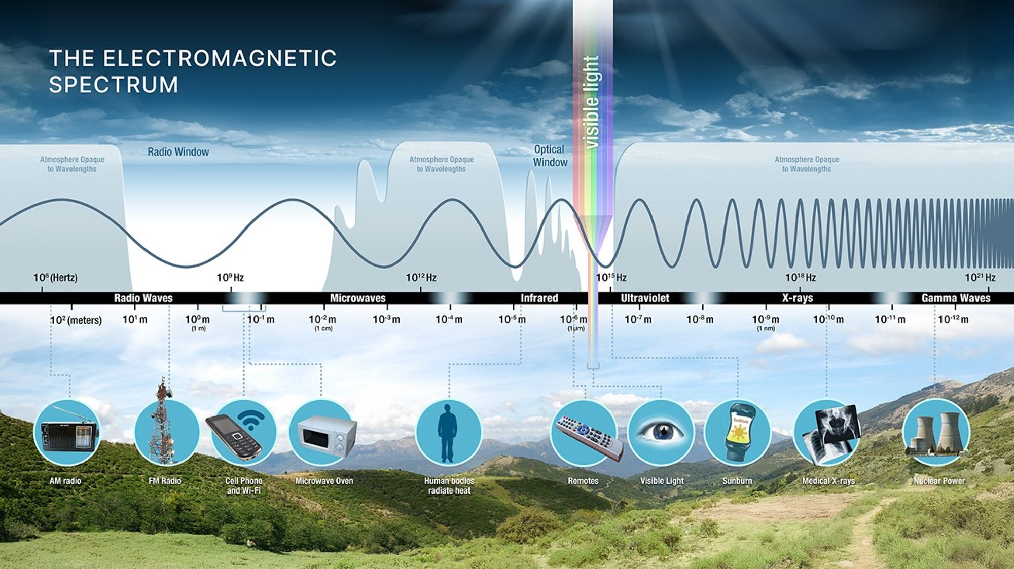
What to notice: Earth is transparent mainly in two windows (optical and radio), so many wavelengths require space telescopes. (Credit: NASA)
Modern Observatories
Ground-based giants:
- Keck (Hawaii): Twin 10m mirrors, optical/infrared
- VLT (Chile): Four 8.2m telescopes, can work together
- ALMA (Chile): 66 radio dishes for millimeter waves
- ELT (under construction): 39m mirror — will be the largest optical telescope
Space telescopes:
- Hubble (1990–present): Optical/UV, iconic images, 2.4m mirror
- JWST (2021–present): Infrared, 6.5m mirror, sees earliest galaxies and exoplanet atmospheres
- Chandra (1999–present): X-rays, hot gas and black holes
- Fermi (2008–present): Gamma rays, extreme cosmic events
The Power of Multi-Wavelength Astronomy
Different wavelengths reveal different physics. A complete picture requires observations across the spectrum — which is why we build telescopes of all kinds.
The same object can look completely different at radio, infrared, visible, X-ray, and gamma-ray wavelengths. Each reveals a different physical process: cold gas, warm dust, starlight, hot plasma, relativistic particles.
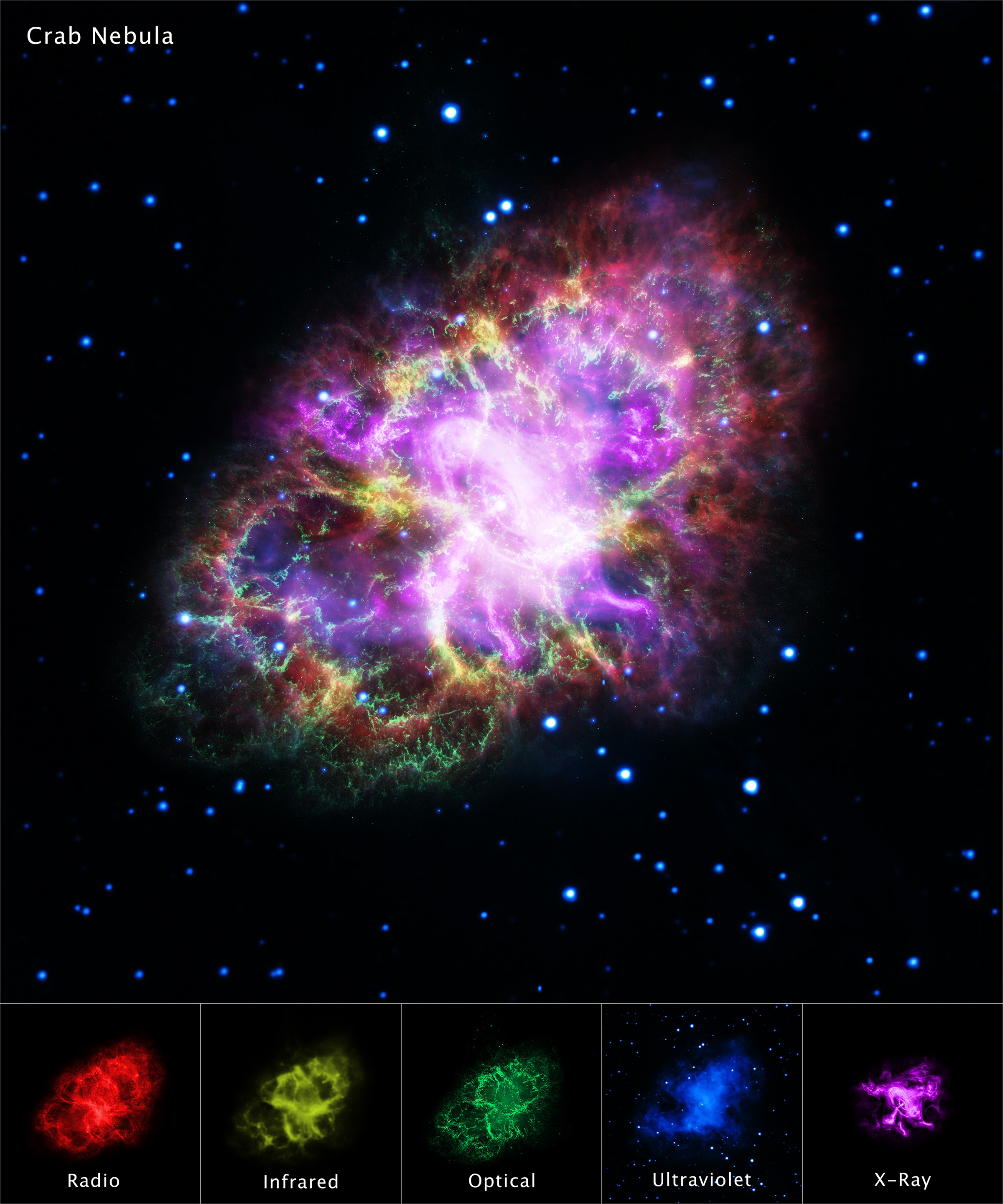
What to notice: The same object can look completely different at different wavelengths; each band highlights different physics. (Credit: NASA/CXC/SAO)
The power of infrared becomes especially clear in side-by-side comparisons. Hubble’s optical view of the Pillars of Creation shows dark, opaque dust columns — but JWST’s infrared vision pierces right through, revealing thousands of newborn stars hidden inside:
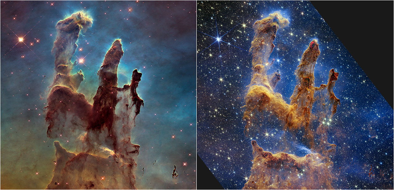
What to notice: Left (Hubble optical)—dark, opaque columns block visible light. Right (JWST infrared)—thousands of embedded newborn stars revealed. Infrared penetrates the dust that blocks optical light. (Credit: Illustration: NASA, ESA, CSA)
The same effect applies to entire galaxies. Compare NGC 1566 in optical light (where dust lanes obscure structure) versus infrared (where the dust becomes transparent):
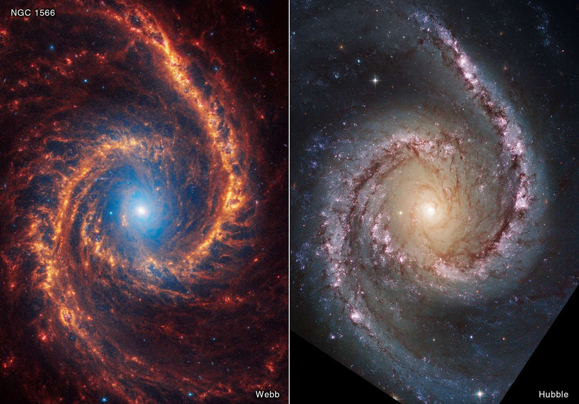
What to notice: the same galaxy can look dramatically different in different bands; dust that hides structure in one band may become transparent in another.
Types of Telescopes (Brief)
Refractors vs. Reflectors
Refractors use lenses to focus light. Limited by chromatic aberration (different wavelengths focus at different points) and lens size/weight. Galileo used a refractor in 1610.
Reflectors use curved mirrors. Can be made much larger; no chromatic aberration. Most modern research telescopes are reflectors. Newton built the first practical reflector in 1668.
Radio Telescopes
Radio waves have wavelengths millions of times longer than visible light. By \(\theta \propto \lambda/D\), radio telescopes need to be enormous to achieve decent resolution. The Arecibo dish (now collapsed) was 305m across; the FAST dish in China is 500m.
To get even better resolution, multiple radio dishes work together (interferometry), effectively creating a telescope the size of their separation. The Event Horizon Telescope, which imaged a black hole’s shadow, uses dishes across the entire Earth!
Interferometry: Combining signals from multiple telescopes to achieve the resolution of a single telescope the size of their separation. Used extensively in radio astronomy.
Doppler Effect:
- \(\Delta\lambda/\lambda_0 = v/c\) measures radial velocity (line-of-sight only)
- Rest wavelength = lab reference. Blueshift = approaching; redshift = receding.
- Blueshift/redshift apply to all wavelengths, not just visible.
- Exoplanets detected via stellar wobble (periodic Doppler shifts)
- Dark matter discovered via flat galaxy rotation curves (stars orbit too fast)
Telescopes:
- Light-gathering power \(\propto\) \(D^2\) (area)
- Resolution: \(\theta \approx 1.22\lambda/D\) (larger D and shorter \(\lambda\) \(\rightarrow\) finer detail)
- Space telescopes access wavelengths blocked by atmosphere
Toolkit Complete — Now We Apply It
With L10 complete, you now have the full astronomer’s toolkit:
| Lecture | Key Insight | What It Reveals |
|---|---|---|
| L1-L2 | Scale of the universe | Our cosmic address |
| L3-L4 | The sky as a map | Coordinates, seasons, phases, eclipses |
| L5-L6 | Motion reveals mass | Orbits \(\rightarrow\) masses (Kepler + Newton) |
| L7-L8 | Light reveals temperature | Blackbody, Wien, Stefan-Boltzmann |
| L9 | Light reveals composition | Spectral lines, OBAFGKM |
| L10 | Light reveals motion | Doppler, exoplanets, dark matter |
| L10 | Telescopes collect light | Light-gathering, resolution, wavelengths |
Your toolkit is complete. Now let’s use it.
Next week (L11–L13) is our capstone week: we apply every tool to the solar system, planetary climates, exoplanets, and the search for life. Think of it as a victory lap that also prepares you for the Module 1 Exam.
Next up: L11 — Our Cosmic Backyard (Solar System Architecture & Formation)
Practice Problems
Solutions are available in the Lecture 10 Solutions.
Core (do these first)
1. Doppler Calculation: A star’s sodium D line (rest wavelength 589.0 nm) is observed at 589.2 nm. Calculate the star’s radial velocity. Is it approaching or receding? (Remember: \(\Delta\lambda > 0\) means receding.)
2. Radial vs. Transverse: A star has a space velocity of 50 km/s, but it’s moving entirely across the sky (perpendicular to our line of sight). What Doppler shift do we measure?
3. Telescope Comparison: Telescope A has a 4m mirror; Telescope B has a 2m mirror. How much more light does A collect? How does A’s resolution compare to B’s (at the same wavelength)?
4. Multi-wavelength Astronomy: Why do astronomers observe the same object at different wavelengths? Give an example of something you’d learn from infrared that you couldn’t learn from visible light alone.
Synthesis
5. Doppler + Wien’s Law: A distant star has its \(H\alpha\) line observed at 656.50 nm (rest wavelength 656.28 nm). Separately, you measure the star’s blackbody peak at \(\lambda_{peak} = 580\) nm. Using Wien’s Law (\(\lambda_{peak} = 2.9 \times 10^6 /T\) with \(\lambda\) in nm and \(T\) in K), determine both the star’s radial velocity and its surface temperature. How do these two measurements use different properties of the same starlight?
Challenge
6. Exoplanet or Binary?: A star’s spectral lines shift with amplitude \(\pm0.005\) nm around a rest wavelength of 500 nm, with a period of 3 days. Calculate the star’s radial velocity amplitude. Is this likely caused by a planet or a stellar companion? Explain your reasoning.
7. Dark Matter: Explain in your own words how galaxy rotation curves provide evidence for dark matter. Use the concepts of orbital velocity, gravity, and mass.
8. Space vs. Ground: The James Webb Space Telescope (JWST) observes in infrared. Why couldn’t we just build a larger infrared telescope on the ground instead of spending billions on a space mission?
Glossary
| Term | Definition |
|---|---|
| Rest wavelength (\(\lambda_0\)) | The wavelength of a line measured in the lab with no relative motion |
| Doppler shift | The change in observed wavelength due to relative motion |
| Radial velocity | The component of velocity along the line of sight |
| Transverse velocity | The component of velocity across the sky (perpendicular to line of sight) |
| Blueshift | Shift to shorter wavelengths (source approaching) |
| Redshift | Shift to longer wavelengths (source receding) |
| Barycentric correction | Correcting for Earth’s orbital motion around the Sun |
| Dark matter | Invisible matter that has gravity but doesn’t interact with light |
| Light-gathering power | A telescope’s ability to collect light; \(\propto\) \(D^{2}\) |
| Angular resolution | Ability to distinguish closely-spaced objects; \(\propto\) \(\lambda /D\) |
| Rayleigh criterion | The formula \(\theta = 1.22\lambda/D\) for diffraction-limited resolution |
| Interferometry | Combining signals from multiple telescopes to achieve higher resolution |
- ★ Angular resolution
- A telescope's ability to distinguish closely-spaced objects; limited by \(\theta \approx 1.22\lambda/D\). Larger aperture and shorter wavelength give finer resolution.
- ★ Blueshift
- A shift to shorter wavelengths, indicating the source is approaching the observer. \(\lambda_{obs} < \lambda_0\); negative \(\Delta\lambda\).
- ★ Doppler effect
- The change in observed wavelength due to relative motion between source and observer. Approaching sources are blueshifted; receding sources are redshifted.
- ◇ Interferometry
- Combining signals from multiple telescopes to achieve the resolution of a single telescope the size of their separation. Used extensively in radio astronomy; enabled imaging of a black hole's shadow.
- ★ Light-gathering power
- A telescope's ability to collect light, proportional to the area of its primary mirror: \(\propto D^2\). Doubling diameter quadruples the light collected.
- ★ Radial velocity
- The component of an object's velocity along the line of sight (toward or away from the observer). This is what Doppler measurements detect; transverse motion produces no Doppler shift.
- ◇ Rayleigh criterion
- The formula \(\theta = 1.22\lambda/D\) for diffraction-limited angular resolution. Sets the fundamental limit; atmospheric seeing often dominates for ground telescopes.
- ★ Redshift
- A shift to longer wavelengths, indicating the source is receding from the observer. \(\lambda_{obs} > \lambda_0\); positive \(\Delta\lambda\).
- ★ Rest wavelength (λ₀)
- The wavelength of a spectral line as measured in the laboratory, with no relative motion. The reference against which Doppler shifts are measured.
- ◇ Transverse velocity
- The component of an object's velocity perpendicular to the line of sight (across the sky). Produces proper motion but no Doppler shift.