Lecture 4: The Last Piece — Weighing Stars

How binary star orbits reveal the most important property in astrophysics

binary-stars

stellar-masses

mass-luminosity

orbits

spectroscopic-binaries

Mass controls a star’s luminosity, temperature, lifetime, and death — but you can’t weigh a star from its light alone. Binary star systems, where two stars orbit a common center of mass, let us apply Newton’s version of Kepler’s third law to measure stellar masses directly. The result — the mass-luminosity relation — reveals that mass is the single most important property of a star.

Author

Dr. Anna Rosen

Published

February 24, 2026

Learning Objectives

After completing this reading, you should be able to:

Explain why mass is the most fundamental stellar property and why it cannot be measured from a single, isolated star’s light alone
Describe visual, spectroscopic, and eclipsing binary systems and explain what each type reveals
Apply Newton’s version of Kepler’s third law ($P^2=\frac{4\pi^2 a^3}{G(M_1+M_2)}$) to determine the total mass of a binary system
Use the center-of-mass condition and radial velocity amplitudes to determine individual masses
Interpret the mass-luminosity relation ($L \propto M^{3.5}$) and explain why it makes mass the “master variable” for main-sequence stars
Connect mass measurement to the full Module 2 inference chain

Concept Throughline

Mass is the most important thing about a star — and the one thing you can’t see. Every other property — luminosity, temperature, radius, lifetime, and how a star dies — follows from mass. But mass leaves no direct imprint on a star’s light. To weigh a star, you need to catch it in a gravitational dance with a partner. Binary stars are nature’s gift to astronomers: two bodies orbiting each other under gravity, revealing their masses through the physics you already know.

Reading Map — Choose Your Track

Track A (Core, ~25 min): Read Parts 1–4 in order — the main text, all worked examples, and Quick Checks. Skip any box marked Enrichment. This gives you every concept and equation you need for homework and exams.

Track B (Full, ~35 min): Read everything, including Enrichment boxes (historical context, inclination effects, mass function). These topics deepen your understanding and connect to research applications.

Both tracks cover all core learning objectives.

The Big Idea

Mass determines a star’s fate — but you can’t weigh a star from its light alone.

In Lectures 1–3, you learned to measure a star’s distance, luminosity, temperature, radius, and composition from photons. But none of these tells you the most consequential property: mass. A star’s mass determines how brightly it shines, how hot its surface is, how long it lives, and how it dies. Yet mass is invisible — no spectral line, no color, no brightness measurement reveals it directly.

What you’ll gain: After this reading, you’ll know how astronomers exploit gravitational physics — specifically, binary star orbits — to measure the one property that controls all the others. And you’ll see that the resulting mass-luminosity relation is the most important empirical relation in stellar astrophysics.

Part 1: The Hidden Variable

Why Mass Matters Most

Consider two stars on the main sequence — the band where most stars spend most of their lives. One has mass $M = 0.5\,M_\odot$; the other has $M = 10\,M_\odot$. How do they compare?

Property	$0.5\,M_\odot$ star	$10\,M_\odot$ star	Ratio
Luminosity	$\sim 0.09\,L_\odot$	$\sim 3 \times 10^3\,L_\odot$	$\sim 3 \times 10^4$
Surface temperature	$\sim 3{,}800\,\text{K}$	$\sim 2.5 \times 10^4\,\text{K}$	$\sim 7$
Radius	$\sim 0.5\,R_\odot$	$\sim 6\,R_\odot$	$\sim 12$
Main-sequence lifetime	$\sim 60\,\text{Gyr}$	$\sim 20\,\text{Myr}$	$\sim 3 \times 10^3$
Spectral type	M	B	—
Death	White dwarf	Core-collapse supernova	—

A factor of 20 in mass increases luminosity by a factor of $3 \times 10^4$, reduces lifetime by a factor of $3 \times 10^3$, and leads to completely different endpoints. Mass is the master variable. Change the mass, and everything else follows.

Mass Detective — Case Opened

The suspect: Mass — controls luminosity, temperature, radius, lifetime, and death. The problem: It has no fingerprint in the light. No spectral line, no color, no brightness reveals it. We need a different kind of evidence. The investigation begins.

Why Mass Is Hidden

So why can’t we just “read” mass from a star’s spectrum, the way we read temperature from spectral type or composition from line wavelengths?

The problem is fundamental: mass affects a star’s light only indirectly, through its influence on internal structure. A star’s spectrum encodes surface properties — temperature, composition, surface gravity. Mass determines those surface properties, but the mapping from mass to surface isn’t unique without a physical model connecting them. A red giant and a red dwarf can have similar surface temperatures but wildly different masses.

Put differently: luminosity, temperature, and composition are observables — properties encoded directly in the photons reaching your detector. Mass is a derived quantity — you need a physical model (or a dynamical measurement) to get it.

The solution is gravity. If a star has a gravitational companion — another star orbiting it — then orbital dynamics gives us the mass directly, through physics you already know from Module 1.

Think First

Before reading further, recall from Module 1 (Lecture 3): Newton showed that Kepler’s third law contains the mass of the central body. For a planet orbiting the Sun, we used $P^2=\frac{4\pi^2 r^3}{GM}$. What changes when both objects have comparable mass — like two stars orbiting each other?

Answer

Replace $M$ with $M_1+M_2$ and replace $r$ with the star-star separation $a$. The binary form is $P^2=\frac{4\pi^2 a^3}{G(M_1+M_2)}$.

Part 2: Binary Stars — Nature’s Mass Laboratories

Most Stars Have Partners

One of the most important facts in stellar astronomy: roughly half of all Sun-like stars are in binary or multiple star systems. For massive stars (O and B types), the binary fraction is even higher — at least $70\%\text{–}90\%$ (Sana et al. 2012). Binary stars are not rare curiosities. They are the norm.

This is fortunate, because binary orbits are the only direct way to measure stellar masses. Without binaries, the mass-luminosity relation — and much of our understanding of stellar physics — would be inaccessible.

So the challenge is clear: how do you weigh something you can’t touch, can’t visit, and whose mass leaves no direct imprint on the light it emits? The answer is to watch it move. If a star has a gravitational partner, Newton’s laws let you convert orbital motion into mass — the same physics you used in Module 1 to weigh the Sun from Earth’s orbit. Astronomers have found three complementary ways to detect and exploit binary orbits, each revealing different pieces of the puzzle. Let’s see what each strategy gives us and what it leaves unknown.

Interactive Demo: Binary Orbits

Before diving in, explore how binary stars orbit their common center of mass — adjust masses, separations, and eccentricities to build intuition for what observers actually see: Binary Orbits Demo

Visual Binaries: Resolved on the Sky

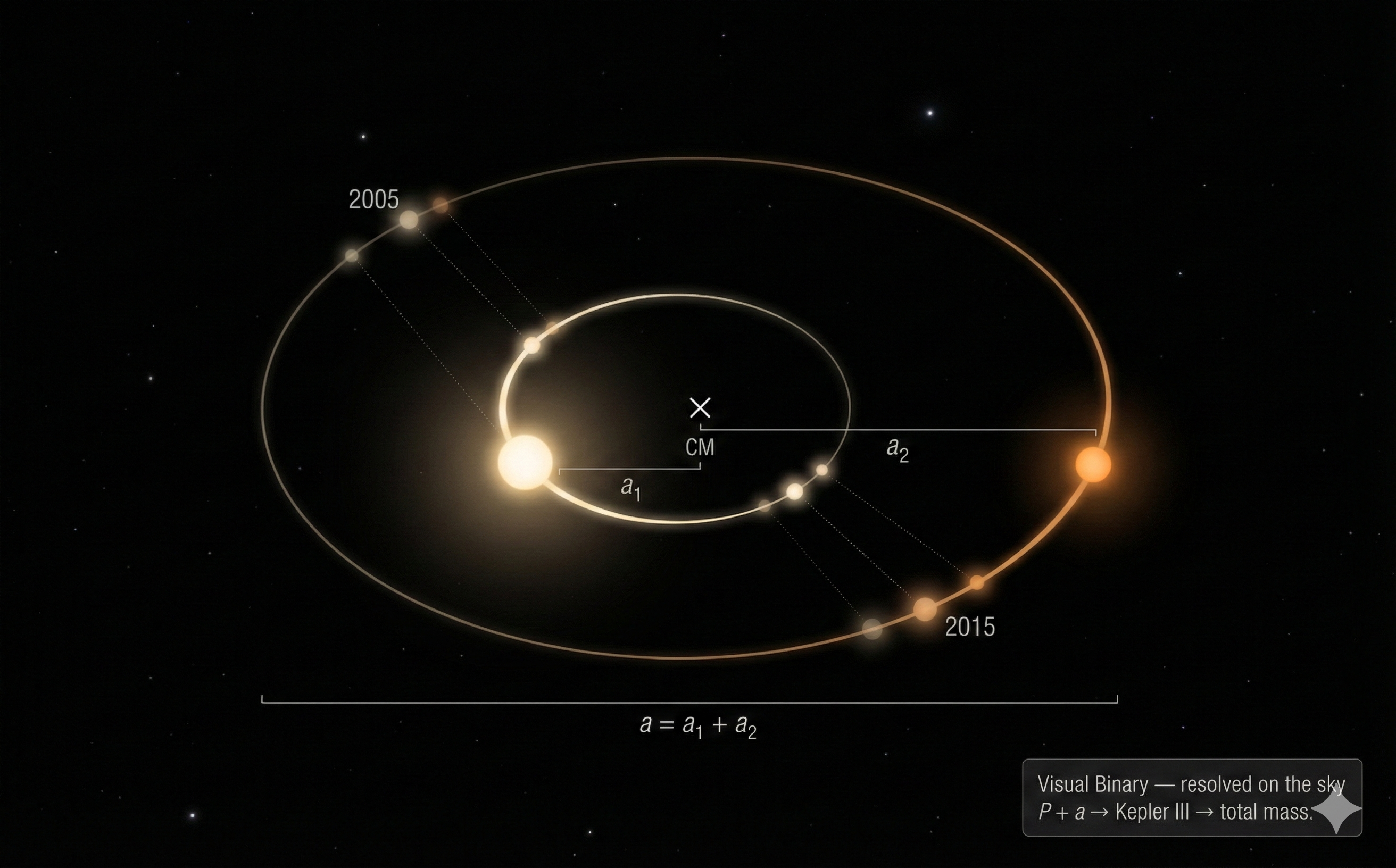
What to notice: Two stars orbit their common center of mass (×). The heavier star (yellow-white) traces a smaller orbit ($a_1$); the lighter star (orange) swings wide ($a_2$). Ghosted positions at different epochs show the decades of patient observation needed to map the orbit. With the period $P$ and physical separation $a = a_1 + a_2$ (which requires knowing the distance), Kepler III yields the total mass. (Credit: ASTR 201 (Gemini))

A visual binary is a pair of stars close enough to us (and far enough apart from each other) that we can resolve both stars as separate points of light through a telescope. By tracking their positions over years or decades, we can map out their orbits on the sky.

What visual binaries give us:

Orbital period $P$ (from watching the orbit repeat)
Angular size of the orbit on the sky (in arcseconds)
If the distance is known (from parallax), the angular orbit converts to a physical separation $a$ in AU or cm
From $P$ and $a$, Kepler’s third law gives the total mass $M_1 + M_2$
If we can track both stars’ orbits around the center of mass, we also get the mass ratio $M_1/M_2$

Note the critical role of distance: Without a parallax measurement (Lecture 1), the angular orbit cannot be converted to a physical separation, and Kepler III cannot yield the mass. Distance — as always — is the master key.

Limitation: Visual binaries require wide separations (long periods — often decades to centuries) and nearby systems. They’re relatively rare in practice.

Classic example: Sirius A and Sirius B, first resolved in 1862. Sirius A is a bright A-type star ($2.06\,M_\odot$); Sirius B is a white dwarf ($1.02\,M_\odot$). Their orbital period is $50.1~\text{yr}$, and the system is only $2.64~\text{pc}$ away, making it one of the best-measured visual binaries.

Enrichment: The Dark Companion of Sirius — A Prediction Vindicated

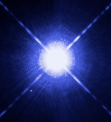
$Hubble Space Telescope image of the Sirius binary system. Sirius A is a brilliant overexposed white star dominating the frame with prominent diffraction spikes. Sirius B is visible as a small faint dot at lower left, separated by several arcseconds.$

Credit: NASA/ESA/HST

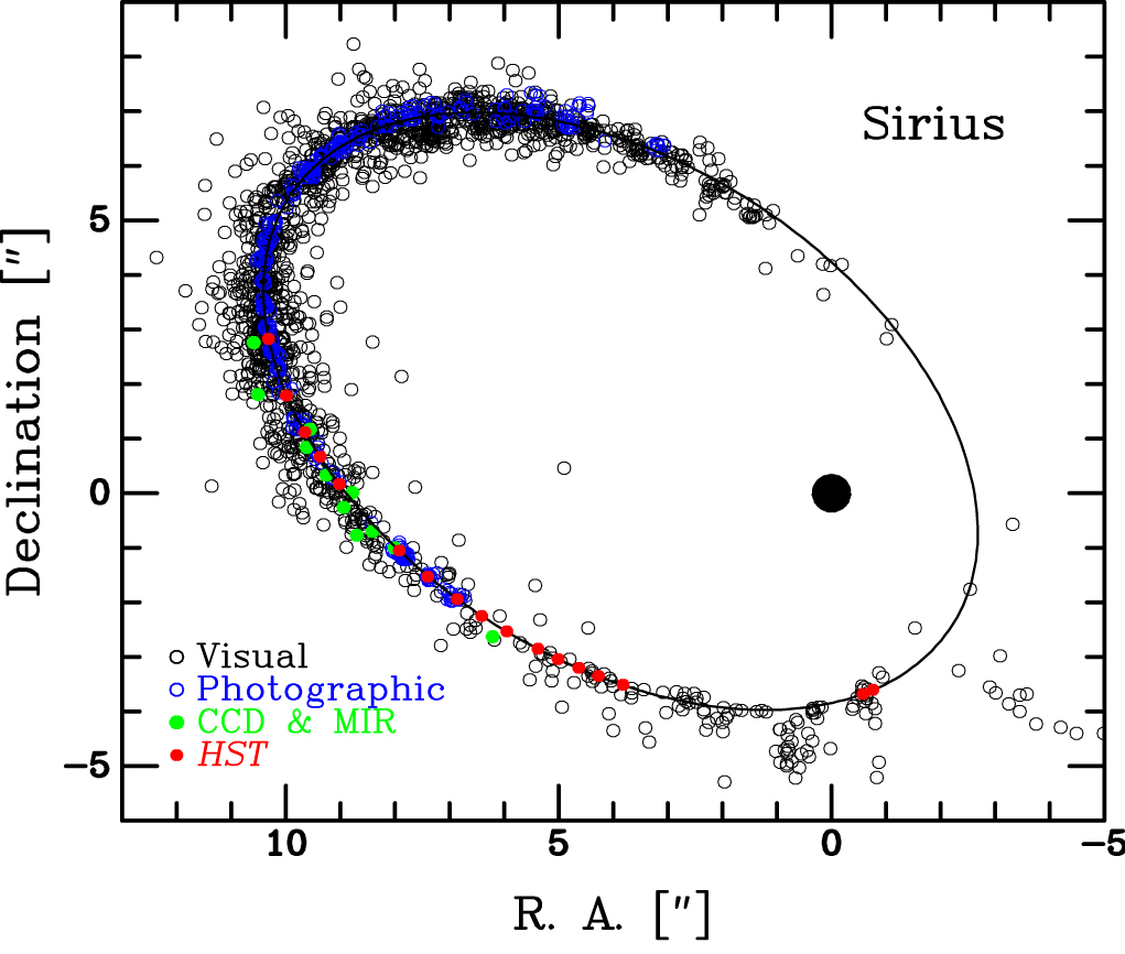
Diagram showing the elliptical orbit of Sirius B around Sirius A, with positions marked at various epochs spanning decades. The orbital ellipse is clearly elongated, with Sirius A near one focus.

Credit: Public domain

In 1844, the mathematician Friedrich Bessel noticed something strange: Sirius, the brightest star in the sky, was not moving in a straight line. Its proper motion across the sky wobbled — as if something invisible were tugging it back and forth. Bessel concluded that Sirius must have an unseen companion, and predicted its orbital period from the wobble.

This was mass measurement by gravitational influence, decades before anyone laid eyes on the companion. In 1862, telescope-maker Alvan Graham Clark spotted a faint point of light near Sirius — exactly where the orbit predicted it should be. That faint dot, Sirius B, turned out to be one of the most extraordinary objects in stellar astronomy: a star with $1.02\,M_\odot$ (nearly the Sun’s mass) crammed into a volume the size of Earth ($R \approx 0.008\,R_\odot$). Its surface temperature is ${\sim}2.5 \times 10^4~\text{K}$ — far hotter than Sirius A — yet its luminosity is only ${\sim}0.03\,L_\odot$. Hot but tiny: a white dwarf.

Sirius B was the first white dwarf ever identified, and its discovery foreshadowed a key theme of this course: the most important stellar properties are often the ones you cannot see directly. Bessel inferred mass from motion — exactly the strategy you are learning in this reading.

Enrichment takeaway: Astrometric wobble can reveal an unseen companion, and orbital dynamics can measure mass before direct imaging confirms the object.

Mass Detective — Clue 1

Watch the sky: If we can see both stars move, we get orbits on the sky → $P$ and $a$ → total mass. But this requires nearby, widely separated pairs — rare and slow. We have one tool. We need more.

Spectroscopic Binaries: Doppler Reveals the Orbit

Most binary stars are too close together and too far from Earth to resolve visually. But we can detect them through the Doppler effect — the very tool you learned in Lecture 3.

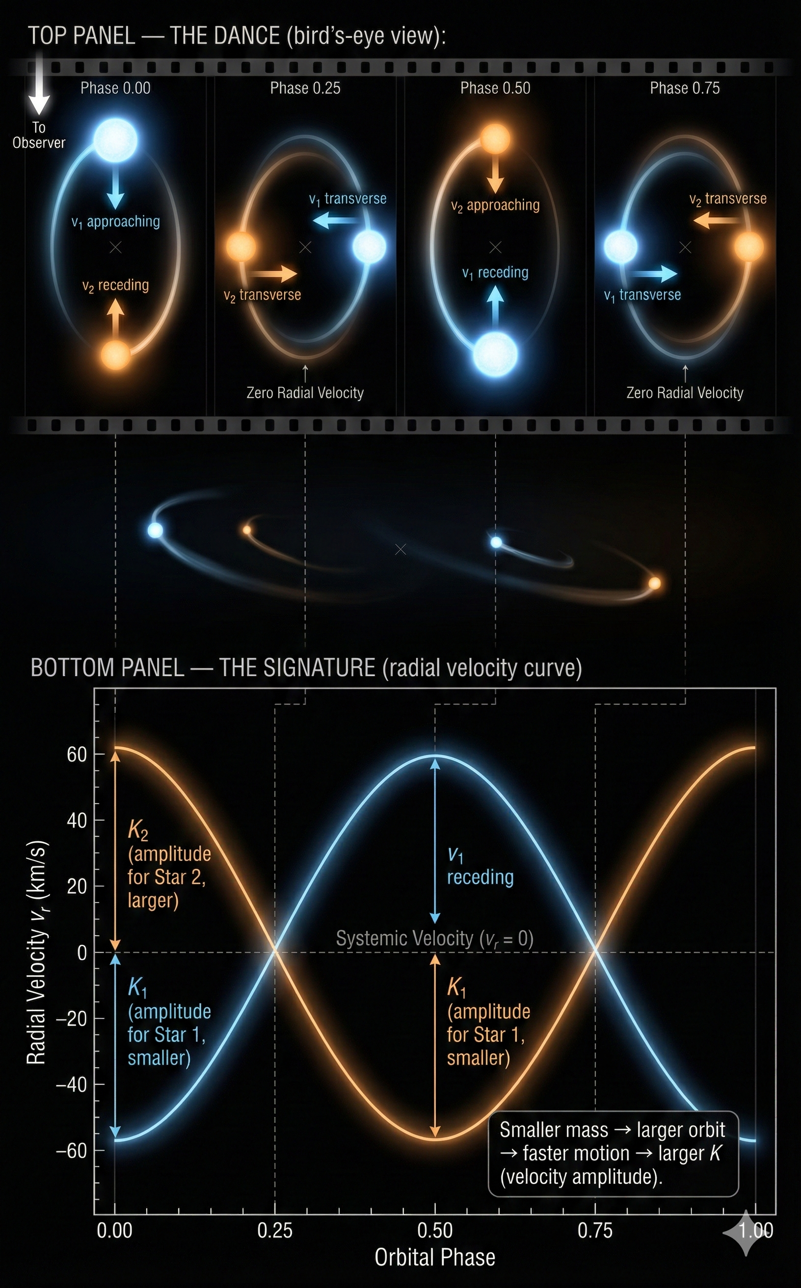
What to notice: Top — the orbital dance seen from above at four phases. Velocity arrows show which star is approaching (blueshift) or receding (redshift) at each moment. Bottom — the radial velocity signature: two sinusoidal curves in anti-phase. The less massive star (orange, $K_2$) has the larger velocity amplitude because it orbits farther from the center of mass and moves faster. The mass ratio comes directly from $M_1/M_2 = K_2/K_1$. (Credit: ASTR 201 (Gemini))

If a star is in a binary system, it orbits the center of mass. During half the orbit, it moves toward us; during the other half, it moves away. Its spectral lines shift back and forth — blueshifted when approaching, redshifted when receding — with a period equal to the orbital period.

A spectroscopic binary is detected by this periodic Doppler wobble. In fact, Lecture 3 already showed you a preview: the worked example of a star with H$\alpha$ oscillating between $656.25~\text{nm}$ and $656.35~\text{nm}$ over $4.0~\text{days}$. That was a spectroscopic binary.

What spectroscopic binaries give us:

Orbital period $P$ (from the Doppler oscillation period)
Radial velocity amplitude $K$ (half the peak-to-peak velocity swing) — directly from the Doppler shift
If both stars’ lines are visible (a double-lined spectroscopic binary, or SB2), we get $K_1$ and $K_2$ for each star separately

Key connection to Lecture 3: The Doppler formula $\Delta\lambda/\lambda_0=v_r/c$ converts wavelength shifts to velocities. Now we use those velocities as a function of time to trace out the orbit.

Single-Lined vs. Double-Lined

In a single-lined spectroscopic binary (SB1), only one star’s lines are visible — the companion is too faint. You get $K_1$ for the brighter star, but not $K_2$. This gives a constraint on the masses but not the individual masses directly (you need additional information).

In a double-lined spectroscopic binary (SB2), both stars’ spectral lines are visible and shift in opposite directions (when star 1 is approaching, star 2 is receding). This gives both $K_1$ and $K_2$, which — combined with $P$ — yields both individual masses.

Mass Detective — Clue 2

Read the Doppler shifts: Periodic wavelength oscillations give $P$ and $K$ — velocity amplitudes that encode the orbit. Works for close pairs at any distance, but we only measure the line-of-sight component. Something is still hidden: the orbital inclination. Two tools now — but a blind spot remains.

Eclipsing Binaries: Light Curves Reveal Geometry

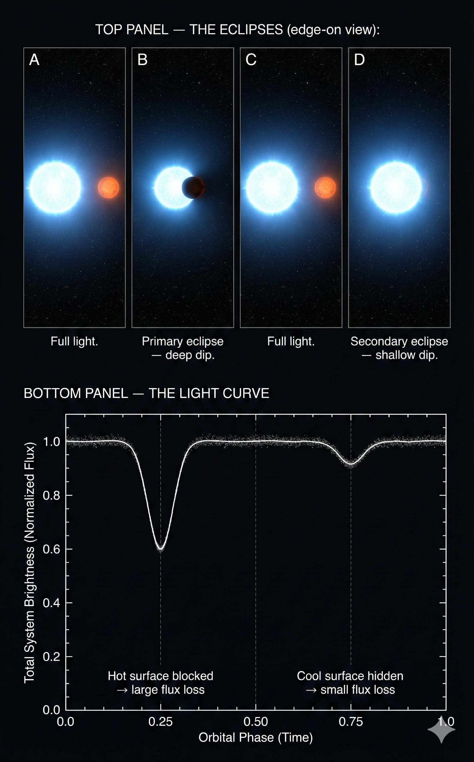
What to notice: Top — an edge-on binary at four phases. When the small cool star transits the hot star (phase B), it blocks high-surface-brightness area → deep dip. When the cool star is hidden behind the hot star (phase D), only its modest contribution is lost → shallow dip. Bottom — the light curve shows both eclipses. The depth ratio encodes the temperature ratio; the duration encodes the stellar radii. (Credit: ASTR 201 (Gemini))

When the orbital plane is nearly edge-on to our line of sight, the stars periodically pass in front of each other. These are eclipsing binaries, and they produce characteristic dips in the combined light — a light curve.

What eclipsing binaries give us:

Orbital period $P$ (from the spacing between eclipses)
Relative stellar radii (from the duration and shape of the eclipses)
Inclination $i \approx 90^\circ$ (the orbit must be nearly edge-on for eclipses to occur)
Temperature ratio (from the relative depths of primary and secondary eclipses)

The last point is particularly valuable: eclipsing binaries tell us the orbital inclination is close to $90^\circ$, which removes the biggest uncertainty in spectroscopic binary measurements (more on this below).

The gold standard: A system that is both an eclipsing binary and a double-lined spectroscopic binary (SB2) gives us everything — period, both velocity amplitudes, inclination, and both radii. These systems provide the most precise stellar mass measurements available: uncertainties of $1\text{–}2\%$.

Classic example: Algol ($\beta$ Persei), one of the first-known eclipsing binaries, dips in brightness every $2.87~\text{days}$ as its cooler companion passes in front of the hot primary.

Mass Detective — Clue 3

Watch the light curve: Eclipses nail down the inclination ($i \approx 90^\circ$) and give us stellar radii as a bonus. Combine Clues 2 + 3 in the same system, and we can measure everything — the gold standard for stellar mass determination. Three complementary tools. The blind spot is closed. Time to extract the masses.

Summary: What Each Type Reveals

Binary Type	How Detected	What It Gives	What It Misses
Visual	Resolved on sky	$P$, $a$ (with distance), mass ratio	Needs decades of observation; nearby only
Spectroscopic	Doppler wobble	$P$, $K_1$ (and $K_2$ if SB2)	Inclination $i$ unknown (only $v \sin i$)
Eclipsing	Light curve dips	$P$, $i \approx 90^\circ$, relative radii, $T$ ratio	Rare geometry (edge-on only)
Eclipsing + SB2	Both	Everything: $M_1$, $M_2$, $R_1$, $R_2$, $T_1/T_2$	Rarest; requires edge-on + bright enough for spectra

Check Yourself

Why can’t you measure a star’s mass from its spectrum alone?
A binary star system has an orbital period of $30~\text{yr}$ and the stars are resolved in a telescope. What type of binary is this?
You observe a star whose H$\alpha$ line oscillates between $656.2~\text{nm}$ and $656.4~\text{nm}$ every $10~\text{days}$. What type of binary is this, and what can you immediately determine?

Answer

A spectrum directly gives surface properties (temperature, composition, surface gravity), not mass itself.
Different masses can produce similar spectra in different evolutionary states (for example, red giants vs red dwarfs).
You need dynamical evidence from orbital motion to measure mass directly.

This is a visual binary.
The stars are spatially resolved, and a $30~\text{yr}$ period is consistent with a relatively wide, directly trackable orbit.

This is a spectroscopic binary, identified by periodic Doppler shifts.
You can immediately measure the period ($P=10~\text{days}$) and the radial-velocity amplitude.
Using half the peak-to-peak line shift, $K=\left(3.0\times10^5~\text{km/s}\right)\left(\frac{0.1~\text{nm}}{656.3~\text{nm}}\right)\approx46~\text{km/s}$.

Argue With a Peer

Your lab partner says: “A star whose spectral lines shift periodically and whose brightness dips periodically — that’s the jackpot. We get everything we need to measure both masses.” Explain why this combination is so powerful. What specific problem does the eclipsing geometry solve that spectroscopy alone cannot?

Answer

Spectroscopy gives $P$, $K_1$, and $K_2$, so you get the mass ratio and $a\sin i$.
Eclipses constrain the geometry to near edge-on, so $i \approx 90^\circ$ and $\sin i \approx 1$.
That removes the $\sin^3 i$ degeneracy, letting you recover true $M_1$ and $M_2$ instead of lower limits.

Why this has to work. For this derivation, we only need two physics ingredients: Newton/Kepler gravity for two-body orbits and the center-of-mass condition that links the two stars. On the observation side, we only need time variation (to get $P$), line-of-sight velocities (to get $K_1$ and $K_2$), and geometry (through inclination $i$). That structure forces a specific chain: $P \rightarrow a$, velocity-amplitude ratio $\rightarrow$ mass ratio, then total mass + mass ratio $\rightarrow$ individual masses. Once those pieces are measured, there is no alternative dynamical route to $M_1$ and $M_2$.

Equation Map: what each measurement buys you

Kepler III $\rightarrow$ total mass from ($P$, $a$)
Doppler $\rightarrow$ $K$’s from line shifts
Center-of-mass $\rightarrow$ mass ratio from $K$ ratio
Inclination $\rightarrow$ $\sin^3(i)$ correction; eclipses remove ambiguity

Part 3: Extracting Masses from Orbits

We now have the observational tools. How do we go from measured quantities ($P$, $K_1$, $K_2$) to stellar masses ($M_1$, $M_2$)? The physics is entirely from Module 1 — Kepler’s third law and Newton’s third law — applied to a two-body system.

Predict First

In a spectroscopic binary, Star 1 has radial velocity amplitude $K_1 = 80~\text{km/s}$ and Star 2 has $K_2 = 200~\text{km/s}$. Both orbit the same center of mass with the same period.

Which star is more massive?
Which star traces a larger orbit around the center of mass?

Commit to answers before reading on. (Hint: think about a seesaw — where does the heavy person sit?)

Answer

Star 1 is more massive because it has the smaller velocity amplitude.
Star 2 traces the larger orbit around the center of mass.
Quantitatively, $\frac{M_1}{M_2}=\frac{K_2}{K_1}=\frac{200}{80}=2.5$.

Step 1: Newton’s Kepler III for Binaries

In Module 1 (Lecture 3), you derived Newton’s version of Kepler’s third law for a planet orbiting a star. The key insight was that the mass of the central body appears in the equation:

\[ P^2 = \frac{4\pi^2\, r^3}{G M} \]

But that assumed the planet’s mass was negligible compared to the star’s ($m \ll M$). In a binary star system, both masses matter. Newton’s full two-body form is:

\[ P^2 = \frac{4\pi^2\, a^3}{G(M_1 + M_2)} \tag{1}\]

Kepler's third law for binary systems

What it predicts
Given the orbital separation $a$ and total mass $M_1 + M_2$, it predicts the orbital period $P$ (or vice versa).

What it depends on
Scales as $P \propto a^{3/2}$ and $P \propto (M_1 + M_2)^{-1/2}$.

What it's saying
Newton's version of Kepler's third law — the *total mass* of a binary system determines how fast the two stars orbit each other at a given separation.

Assumptions

Approximately circular orbits (eccentricity $e \approx 0$)
Newtonian gravity
Both masses contribute — this is the full two-body version

See: the equation

where:

$P$ is the orbital period
$a = a_1 + a_2$ is the total orbital separation (the semi-major axis of the relative orbit)
$M_1$ and $M_2$ are the two stellar masses
$G = 6.67 \times 10^{-8}~\text{cm}^3\,\text{g}^{-1}\,\text{s}^{-2}$ is Newton’s gravitational constant

What changed from the planetary case? Two things: (1) $M$ became $M_1 + M_2$, because both bodies contribute to the gravitational interaction, and (2) $r$ became $a$, the total separation between the two stars (not the distance from either star to the center of mass).

Unit Check

\[ [P^2] = \frac{[\text{cm}^3]}{[\text{cm}^3\,\text{g}^{-1}\,\text{s}^{-2}][\text{g}]} = \frac{\text{cm}^3}{\text{cm}^3\,\text{s}^{-2}} = \text{s}^2\ \checkmark \]

Rearranging for total mass:

\[ M_1 + M_2 = \frac{4\pi^2\, a^3}{G\, P^2} \]

If we measure $P$ and $a$, we get the total mass of the system. But we still need to separate $M_1$ from $M_2$.

What we gained: A direct expression for the total system mass $M_1 + M_2$ from orbital size and period.

Step 2: The Center-of-Mass Condition

Both stars orbit the center of mass of the system — the balance point where the gravitational pulls are equal. Newton’s third law guarantees this: if star 1 pulls on star 2 with force $F$, then star 2 pulls on star 1 with force $F$ in the opposite direction. Both accelerate, but the more massive star has a smaller orbit.

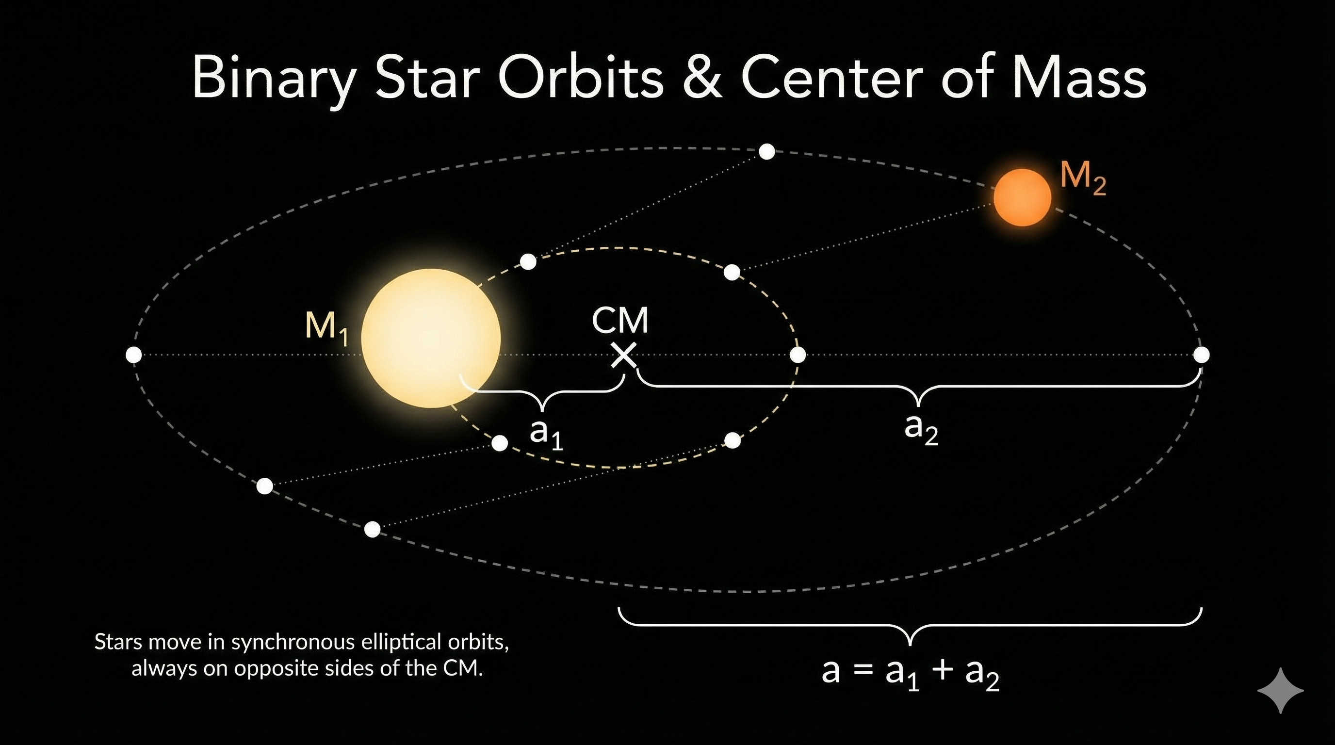
What to notice: The center of mass (×) is the pivot point — always closer to the heavier star. $M_1$ barely moves ($a_1$ small); $M_2$ swings wide ($a_2$ large). The balance condition $M_1 a_1 = M_2 a_2$ means the mass ratio equals the inverse ratio of orbital sizes. Epoch dots show the stars always on opposite sides of the CM. (Credit: ASTR 201 (Gemini))

The center-of-mass condition is:

\[ M_1\, a_1 = M_2\, a_2 \tag{2}\]

Center-of-mass condition (binary)

What it predicts
Given the two masses $M_1$ and $M_2$, it predicts the ratio of their orbital radii $a_1/a_2$.

What it depends on
The more massive star orbits closer to the center of mass: $a_1/a_2 = M_2/M_1$.

What it's saying
Newton's third law in action — both stars orbit the center of mass, but the heavier star has a smaller orbit.

Assumptions

Isolated two-body system
No external forces

See: the equation

where $a_1$ is star 1’s distance from the center of mass, and $a_2$ is star 2’s distance from the center of mass. This means:

\[ \frac{M_1}{M_2} = \frac{a_2}{a_1} \]

The mass ratio equals the inverse ratio of orbital radii. The heavier star has the smaller orbit — it barely moves, while the lighter star swings wide around it.

What we gained: A second independent constraint, the mass ratio $\frac{M_1}{M_2}$, that tells us which star is heavier and by how much.

Step 3: Connecting Velocities to Orbits

For spectroscopic binaries, we don’t measure $a_1$ and $a_2$ directly — we measure velocities. For circular orbits, each star’s orbital speed is:

\[ \begin{aligned} v_1 &= \frac{2\pi\, a_1}{P} \\ v_2 &= \frac{2\pi\, a_2}{P} \end{aligned} \]

Since the period $P$ is the same for both stars (they orbit together), the velocity ratio equals the orbit-size ratio:

\[ \frac{v_1}{v_2} = \frac{a_1}{a_2} = \frac{M_2}{M_1} \]

In practice, what we measure from Doppler shifts are the radial velocity amplitudes $K_1$ and $K_2$ — the maximum line-of-sight velocities. For an orbit with inclination $i$ (where $i = 90^\circ$ is edge-on and $i = 0^\circ$ is face-on), the amplitudes satisfy $K_1=v_1\sin i,\;K_2=v_2\sin i$.

The ratio of $K_1$ to $K_2$ is independent of $i$ (the $\sin i$ cancels):

\[ \frac{M_1}{M_2} = \frac{K_2}{K_1} \]

This is powerful: the mass ratio comes directly from the velocity ratio, regardless of the orbital inclination.

What we gained: A way to compute the mass ratio from observables ($K_1$, $K_2$) without needing $i$.

Step 4: Putting It All Together

For a double-lined spectroscopic binary (SB2) — where we measure $P$, $K_1$, and $K_2$ — we can determine both masses if we know the inclination $i$.

From the velocities and period, the orbital radii are:

\[ \begin{aligned} a_1 \sin i &= \frac{K_1\, P}{2\pi} \\ a_2 \sin i &= \frac{K_2\, P}{2\pi} \end{aligned} \]

The total separation (projected):

\[ a \sin i = (a_1 + a_2) \sin i = \frac{(K_1 + K_2)\, P}{2\pi} \]

Substituting into Kepler’s third law:

\[ \begin{aligned} M_1 + M_2 &= \frac{4\pi^2\,(a \sin i)^3}{G\, P^2 \sin^3 i} \\ &= \frac{(K_1 + K_2)^3\, P}{2\pi\, G\, \sin^3 i} \end{aligned} \]

Combined with the mass ratio $M_1/M_2 = K_2/K_1$, we can solve for each mass individually.

What we gained: A complete pipeline from observables ($P$, $K_1$, $K_2$, $i$) to both individual stellar masses.

Before treating inclination as a nuisance parameter, pause on the geometry. The measured Doppler amplitude is a projected speed, $K=v\sin i$, so each velocity carries one factor of $\sin i$. The same projection propagates into the orbital scale as $a\sin i$ when we infer size from $K$ and $P$. Because Kepler depends on the cube of separation, the projection appears as a cubic correction, $\sin^3 i$, in the inferred mass.

The Inclination Problem

Notice the $\sin^3 i$ in the denominator. If we don’t know the inclination angle $i$, we can only determine $M \sin^3 i$ — a lower limit on the mass. For a face-on orbit ($i = 0^\circ$), there’s no radial velocity at all. For an edge-on orbit ($i = 90^\circ$, $\sin i = 1$), we get the true mass.

Solution 1: If the system is also an eclipsing binary, we know $i \approx 90^\circ$ — problem solved.

Solution 2: For a large sample of randomly oriented binaries, $\langle \sin^3 i \rangle \approx 0.59$ — the average statistical correction factor.

Worked Example: Weighing a Spectroscopic Binary

Problem: An eclipsing, double-lined spectroscopic binary has:

Orbital period: $P = 3.00~\text{days} = 2.59 \times 10^5~\text{s}$
Star 1 radial velocity amplitude: $K_1 = 80~\text{km/s} = 8.0 \times 10^6~\text{cm/s}$
Star 2 radial velocity amplitude: $K_2 = 200~\text{km/s} = 2.0 \times 10^7~\text{cm/s}$
Inclination: $i = 90^\circ$ (eclipsing), so $\sin i = 1$

Find the individual masses $M_1$ and $M_2$.

Solution:

Step 1 — Mass ratio from velocity ratio.

\[\frac{M_1}{M_2} = \frac{K_2}{K_1} = \frac{200~\text{km/s}}{80~\text{km/s}} = 2.5\]

Star 1 is 2.5 times more massive than star 2. (The more massive star moves slower — it’s closer to the center of mass.)

Step 2 — Total separation from velocities and period.

\[ \begin{aligned} a &= a_1 + a_2 \\ &= \frac{(K_1 + K_2)\, P}{2\pi} \\ &= \frac{(8.0 \times 10^6 + 2.0 \times 10^7)~\text{cm/s} \times 2.59 \times 10^5~\text{s}}{2\pi} \end{aligned} \]

\[ \begin{aligned} a &= \frac{2.8 \times 10^7~\text{cm/s} \times 2.59 \times 10^5~\text{s}}{6.28} \\ &= \frac{7.25 \times 10^{12}~\text{cm}}{6.28} \\ &= 1.15 \times 10^{12}~\text{cm} \end{aligned} \]

For reference: $1~\text{AU} = 1.50 \times 10^{13}~\text{cm}$, so $a \approx 0.077~\text{AU}$ — a tight orbit.

Step 3 — Total mass from Kepler’s third law.

\[ \begin{aligned} M_1 + M_2 &= \frac{4\pi^2\, a^3}{G\, P^2} \\ &= \frac{4\pi^2 \times (1.15 \times 10^{12}~\text{cm})^3}{(6.67 \times 10^{-8}~\text{cm}^3\,\text{g}^{-1}\,\text{s}^{-2}) \times (2.59 \times 10^5~\text{s})^2} \end{aligned} \]

Numerator: $4\pi^2 \times 1.52 \times 10^{36}~\text{cm}^3 = 6.01 \times 10^{37}~\text{cm}^3$

Denominator: $6.67 \times 10^{-8} \times 6.71 \times 10^{10} = 4.47 \times 10^{3}~\text{cm}^3\,\text{g}^{-1}$

\[M_1 + M_2 = \frac{6.01 \times 10^{37}}{4.47 \times 10^{3}}~\text{g} = 1.34 \times 10^{34}~\text{g}\]

Convert to solar masses: $M_\odot = 1.99 \times 10^{33}~\text{g}$

\[M_1 + M_2 = \frac{1.34 \times 10^{34}~\text{g}}{1.99 \times 10^{33}~\text{g}} = 6.7\,M_\odot\]

Step 4 — Individual masses from mass ratio.

From $M_1/M_2 = 2.5$ and $M_1 + M_2 = 6.7\,M_\odot$:

\[M_2 = \frac{6.7\,M_\odot}{1 + 2.5} = \frac{6.7}{3.5}\,M_\odot = 1.9\,M_\odot\]

\[M_1 = 2.5 \times 1.9\,M_\odot = 4.8\,M_\odot\]

Unit check: We started with cm, s, and $G$ in CGS → got grams → converted to $M_\odot$. $\checkmark$

Sanity check: Star 1 ($K_1 = 80~\text{km/s}$) moves slower → heavier → $4.8\,M_\odot$. Star 2 ($K_2 = 200~\text{km/s}$) moves faster → lighter → $1.9\,M_\odot$. A $4.8\,M_\odot$ star would be a late B-type star — consistent with being the brighter component. $\checkmark$

The Scaling Approach: Using Solar Units

The worked example above used full CGS arithmetic — instructive but laborious. In practice, astronomers use a scaling version of Kepler’s third law that avoids large numbers entirely.

For the Sun-Earth system: $P_\oplus = 1~\text{yr}$, $a_\oplus = 1~\text{AU}$, $M_\odot + M_\oplus \approx M_\odot$. So:

\[ (1~\text{yr})^2 = \frac{4\pi^2\,(1~\text{AU})^3}{G\,M_\odot} \]

Dividing the binary equation by this:

\[ \left(\frac{P}{1~\mathrm{yr}}\right)^2 = \frac{(a/\mathrm{AU})^3}{(M_1 + M_2)/M_\odot} \]

or equivalently:

\[ \frac{M_1 + M_2}{M_\odot} = \frac{(a/\text{AU})^3}{(P/\text{yr})^2} \tag{3}\]

Kepler's third law (solar units)

What it predicts
Given the orbital separation $a$ (in AU) and period $P$ (in yr), it predicts the total mass $M_1 + M_2$ in solar masses — no constants needed.

What it depends on
Scales as $M_{\text{total}} \propto a^3$ and $M_{\text{total}} \propto P^{-2}$.

What it's saying
The astronomer's working form of Kepler III — all constants absorbed into the choice of solar/AU/yr units. If $a$ in AU and $P$ in yr, the answer comes out in $M_\odot$ automatically.

Assumptions

Same physics as Kepler III for binaries — this is a unit-scaling convenience, not a different equation
Valid for any binary orbit (stellar, planetary) when using AU, yr, $M_\odot$
Approximately circular orbits

See: the equation

This is the astronomer’s working version of Kepler III. All the constants ($4\pi^2$, $G$) are absorbed into the choice of units. If you measure $a$ in AU and $P$ in years, you get total mass in solar masses — no calculator needed for order-of-magnitude work.

Check Yourself: Scaling Kepler III

A visual binary has period $P = 50~\text{yr}$ and semimajor axis $a = 20~\text{AU}$. What is the total mass?
Two equal-mass stars orbit each other with $P = 1~\text{yr}$ at separation $a = 1~\text{AU}$. What is each star’s mass?
If you double the orbital separation while keeping the total mass fixed, by what factor does the period increase?

Answer

$\displaystyle M_1+M_2=\frac{a^3}{P^2}\,M_\odot=\frac{20^3}{50^2}\,M_\odot=\frac{8000}{2500}\,M_\odot=3.2\,M_\odot$.
$\displaystyle M_1+M_2=\frac{1^3}{1^2}\,M_\odot=1.0\,M_\odot$. With equal masses, $M_1=M_2=0.5\,M_\odot$.
$P^2\propto a^3 \Rightarrow P\propto a^{3/2}$, so doubling $a$ gives $P\to2^{3/2}P\approx2.83P$.

Enrichment: The Mass Function (SB1 Systems)

What if only one star’s lines are visible — a single-lined spectroscopic binary (SB1)? You measure $P$ and $K_1$, but not $K_2$. Can you still learn anything about mass?

Yes, but you get a combination called the mass function:

\[ f(M_2) = \frac{M_2^3 \sin^3 i}{(M_1 + M_2)^2} = \frac{K_1^3\, P}{2\pi\, G} \]

The right side is entirely measured quantities. The left side contains three unknowns ($M_1$, $M_2$, $i$). So the mass function is a lower limit on $M_2$ (since $\sin i \leq 1$ and the left side is maximized when $M_1 \to 0$).

If you have an independent estimate of $M_1$ (e.g., from its spectral type), you can constrain $M_2$ more tightly. This technique is how astronomers discovered some of the first stellar-mass black holes — the unseen companion was too massive to be a neutron star.

Enrichment takeaway: SB1 systems do not give individual masses directly, but the mass function provides a robust lower bound on the unseen companion mass.

We now have multiple techniques for measuring stellar masses — visual binaries, spectroscopic binaries, eclipsing systems, and combinations thereof. Over more than a century, astronomers have applied them to hundreds of systems, with the tightest constraints coming from eclipsing SB2 binaries. At this point, the dynamical problem is solved: mass is no longer hidden if the orbit is measured well. That flips the scientific question. Instead of asking how to measure mass, we can now ask what mass controls once measured across many stars.

Part 4: The Mass-Luminosity Relation — The Empirical Payoff

Predict First

You know that the Sun ($1\,M_\odot$) has $L = 1\,L_\odot$. Suppose a main-sequence star has twice the Sun’s mass. How much more luminous do you think it is?

1. $2\times$ brighter (luminosity proportional to mass)
1. $4\times$ brighter (luminosity proportional to mass squared)
1. Something much larger — $10\times$ or more

Commit to a guess before reading on. Most students guess (a) or (b). The actual answer may surprise you.

Answer

Correct choice: (c).
Using $\frac{L}{L_\odot}\approx\left(\frac{M}{M_\odot}\right)^{3.5}$ with $M=2\,M_\odot$, we get $L\approx2^{3.5}L_\odot\approx11\,L_\odot$.
Doubling mass raises luminosity by about an order of magnitude, not by $2\times$ or $4\times$.

Building the Relation from Data

Astronomers have spent over a century measuring masses of binary stars. For each system where individual masses can be determined, the star’s luminosity is also measured (from its apparent brightness and distance). You might expect the results to be messy — after all, stars differ in composition, age, rotation, and evolutionary state. With so many variables, surely mass alone can’t predict luminosity?

It can. When you plot these data — mass on the horizontal axis, luminosity on the vertical axis, both in solar units, both on logarithmic scales — the scatter everyone expected simply isn’t there. Instead, main-sequence stars fall on a remarkably tight relation.

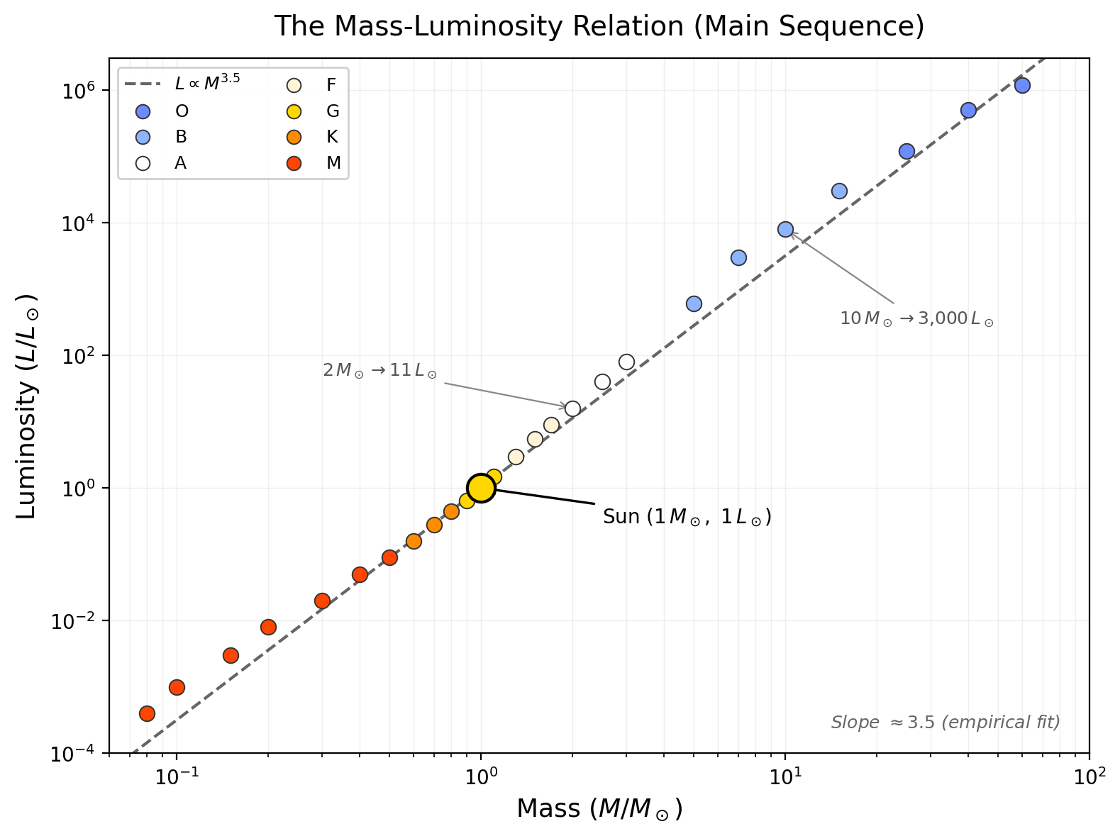
What to notice: Main-sequence stars follow a tight power law $L \propto M^{3.5}$ — a modest increase in mass produces a dramatic increase in luminosity. The Sun sits in the middle. This relation, built entirely from binary star mass measurements, proves that mass is the master variable. (Credit: ASTR 201 (generated))

The idealized power law captures the trend, but real data have scatter. The figure below shows actual measurements from binary star studies:

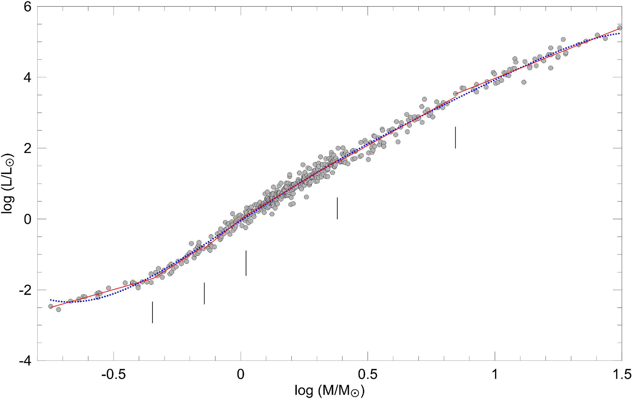
What to notice: Real mass-luminosity data from 509 binary star components with dynamically measured masses. Each gray circle is one star. The red solid line is a piecewise four-segment power-law fit; the blue dotted line is the classical single power law. Vertical tick marks show the mass boundaries between segments. The relation steepens at high masses ($L \propto M^{\sim 4}$) and flattens at low masses ($L \propto M^{\sim 2.3}$). Scatter increases above $\sim 3\,M_\odot$ where stellar evolution is faster. (Credit: Eker et al. 2018, MNRAS 479, 5491)

Main-sequence stars fall on a tight power law:

\[ \frac{L}{L_\odot} \approx \left(\frac{M}{M_\odot}\right)^{3.5} \tag{4}\]

Mass-luminosity relation (main sequence)

What it predicts
Given a main-sequence star's mass $M$, it predicts its luminosity $L$ (approximately).

What it depends on
Scales as $L \propto M^{3.5}$ — a steep power law.

What it's saying
Mass is the master variable for main-sequence stars. Doubling the mass increases luminosity by roughly $2^{3.5} \approx 11\times$.

Assumptions

Star is on the main sequence (core hydrogen burning)
Exponent $\approx 3.5$ is an approximation — actual slope varies from $\sim 2.3$ for $M < 0.43\,M_\odot$ to $\sim 4$ for $M > 2\,M_\odot$
Empirical relation derived from binary star mass measurements

See: the equation

This exponent is why the main sequence is not just a temperature sequence or a luminosity sequence, but a mass sequence in disguise. A small shift in mass produces a disproportionate shift in luminosity, so tiny horizontal moves in mass correspond to huge vertical consequences in emitted power. In other words, the exponent is the lever arm that amplifies mass differences into the large astrophysical contrasts you observe. That is why this relation does more than fit a plot — it governs downstream physics. In Module 3, the same leverage will reappear in evolution: timescales and stellar endpoints trace back to how sharply luminosity responds to mass.

The exponent $3.5$ is an approximation — the actual relationship is slightly steeper at high masses (${\sim}4$ for $M > 2\,M_\odot$) and shallower at low masses (${\sim}2.3$ for $M < 0.43\,M_\odot$). But $3.5$ captures the essential behavior across a wide range.

What the Relation Tells Us

The steepness of the mass-luminosity relation is the key. A modest change in mass produces a dramatic change in luminosity:

Mass ($M_\odot$)	$L/L_\odot \approx (M/M_\odot)^{3.5}$	Factor relative to Sun
$0.1$	$0.1^{3.5} = 3.2 \times 10^{-4}$	$3 \times 10^3$ times fainter
$0.5$	$0.5^{3.5} = 0.088$	$11$ times fainter
$1.0$	$1.0$	$1$ (the Sun)
$2.0$	$2.0^{3.5} = 11.3$	$11$ times brighter
$10$	$10^{3.5} = 3.16 \times 10^3$	$\sim 3 \times 10^3$ times brighter
$50$	$50^{3.5} = 8.8 \times 10^5$	$\sim 10^6$ times brighter

Did your prediction land?

If you guessed “(a) $2\times$” in the Predict First prompt, you’re off by a factor of 5. The answer is (c): a $2\,M_\odot$ star is $2^{3.5} \approx 11\times$ brighter than the Sun. The universe is fiercely nonlinear. Small changes in mass produce enormous changes in luminosity — and this has profound consequences for stellar lifetimes.

The full range of main-sequence masses (${\sim}0.08\,M_\odot$ to ${\sim}150\,M_\odot$) spans about three orders of magnitude — a factor of ${\sim}2 \times 10^3$ in mass. But the luminosity range spans ten orders of magnitude — a factor of ${\sim}10^{10}$!

Why Mass Controls Lifetime

Once luminosity scales this steeply with mass, lifetime becomes an exponent game.

Here’s a beautiful consequence. A star’s hydrogen fuel available for nuclear fusion scales roughly with its total mass $M$. Its luminosity — the rate at which it burns that fuel — scales as $M^{3.5}$, so $t_{\rm MS}\propto M/L\propto M^{-2.5}$.

More massive stars live much shorter lives. The Sun’s main-sequence lifetime is about $10~\text{Gyr}$. A $10\,M_\odot$ star: $t \sim 10 \times 10^{-2.5}~\text{Gyr} \approx 30~\text{Myr}$ — roughly 300 times shorter. A $0.5\,M_\odot$ star: $t \sim 10 \times 0.5^{-2.5}~\text{Gyr} \approx 57~\text{Gyr}$.

Pause on that last number. The universe is $13.8~\text{Gyr}$ old. A $0.5\,M_\odot$ red dwarf born at the Big Bang is not even a quarter of the way through its main-sequence life. Every low-mass star that has ever formed is still shining today. Not a single one has died of old age. The graveyard of stellar evolution contains only the remains of massive stars — the ones that burned bright and fast.

Connection: Mass as the Master Variable

This is why mass is the single most important property of a star:

Luminosity follows from mass: $L \propto M^{3.5}$
Temperature follows from mass (through stellar structure)
Radius follows from $L$ and $T$: $R \propto L^{1/2} T^{-2}$ (Stefan-Boltzmann)
Lifetime follows from mass: $t \propto M^{-2.5}$
Death follows from mass: low mass → white dwarf; high mass → supernova → neutron star or black hole

Know the mass, predict the fate. This is why the mass-luminosity relation is the single most important empirical relation in stellar astrophysics — and why binary stars, which give us masses, are so precious.

Mass Detective — Case Closed

Evidence summary: Visual binaries gave us orbits on the sky (Clue 1). Spectroscopic binaries gave us Doppler velocities (Clue 2). Eclipsing binaries removed the inclination ambiguity (Clue 3). Together, they let us weigh stars using Newton’s and Kepler’s laws.

The verdict: Mass is the master variable. $L \propto M^{3.5}$ means a star’s mass determines its luminosity, temperature, radius, lifetime, and death. The suspect has been identified — and it controls everything.

Case status: Closed. But the investigation continues in Lecture 5 — when we plot all these measurements on one diagram and discover that mass organizes the entire pattern.

Check Yourself

Using the mass-luminosity relation, estimate the luminosity of a $5\,M_\odot$ main-sequence star in solar luminosities.
Estimate the main-sequence lifetime of a $5\,M_\odot$ star, given that the Sun’s is ${\sim}10~\text{Gyr}$.
Two main-sequence stars have luminosities $L_A = 100\,L_\odot$ and $L_B = 0.01\,L_\odot$. Estimate the ratio of their masses.
Why does the mass-luminosity relation apply only to main-sequence stars and not to giants or white dwarfs?

Answer

$\displaystyle L\approx5^{3.5}L_\odot=5^3\cdot5^{0.5}L_\odot=125\times2.24\,L_\odot\approx280\,L_\odot$.
$\displaystyle t_{\rm MS}\approx10~\text{Gyr}\times5^{-2.5}=\frac{10}{5^{2.5}}~\text{Gyr}\approx\frac{10}{56}~\text{Gyr}\approx0.18~\text{Gyr}=180~\text{Myr}$.
$\displaystyle \frac{M_A}{M_B}=\left(\frac{L_A}{L_B}\right)^{1/3.5}=\left(\frac{100}{0.01}\right)^{1/3.5}=(10^4)^{0.286}\approx14$.

The $L\propto M^{3.5}$ relation is calibrated for main-sequence stars in hydrogen-burning equilibrium.
Giants are evolved stars, so luminosity depends strongly on structure and evolutionary stage, not only mass.
White dwarfs are cooling remnants, so luminosity comes from stored thermal energy, not ongoing core fusion.

Observable → Model → Inference: The Binary Star Chain

Let’s trace the full O→M→I framework for binary star mass measurement:

Observable: Periodic shifts in spectral line wavelengths (Doppler oscillation). In eclipsing systems: periodic brightness dips.

Model: Two stars orbiting a common center of mass under Newtonian gravity. Kepler’s third law connects orbital parameters to total mass. Newton’s third law connects the center of mass to the mass ratio.

Inference: From the period $P$ and velocity amplitudes $K_1$, $K_2$: the individual stellar masses $M_1$ and $M_2$. From a large sample: the mass-luminosity relation — the most important empirical scaling in stellar astrophysics.

graph TD
  O1["Observable: spectral line wavelength shifts vs time"]
  O2["Observable: light-curve dips vs time (if eclipsing)"]
  O3["Observable: astrometric positions vs time (visual branch)"]
  Q["Measured quantities: P, K1, K2, i (if eclipsing), a (if visual + distance)"]
  M["Model: Newtonian two-body orbit + center of mass"]
  I1["Infer orbital scale: a or a sin i"]
  I2["Infer dynamical outputs: M_total and M1/M2"]
  I3["Infer individual masses: M1, M2"]
  I4["Then: L ∝ M^3.5 → t_MS ∝ M^-2.5 → stellar fate"]

  O1 --> Q
  O2 --> Q
  O3 --> Q
  Q --> M
  M --> I1 --> I2 --> I3 --> I4

Connection: The Module 2 Inference Chain — Complete

Each lecture in Module 2 has added one link. The chain is now complete:

Lecture	Tool	Question Answered	What It Unlocks
1	Parallax → distance	How far?	Distance $d$; then luminosity $L = 4\pi d^2 F$
2	Color/flux → temperature; Stefan-Boltzmann	How hot? How big?	Temperature $T$; radius $R$ from $L$ and $T$
3	Spectral lines → composition, Doppler	What’s it made of? How is it moving?	Composition; radial velocity $v_r$
4	Binary orbits → mass	*How heavy?*	Mass $M$; mass-luminosity relation

Combined: From photons alone, we can now characterize every fundamental stellar property — distance, luminosity, temperature, radius, composition, and mass. Next time: We put everything on one diagram — the HR diagram — and discover that the patterns it reveals demand a physical explanation.

Practice Problems

Useful constants: $G = 6.67 \times 10^{-8}~\text{cm}^3\,\text{g}^{-1}\,\text{s}^{-2}$, $M_\odot = 1.99 \times 10^{33}~\text{g}$, $L_\odot = 3.828 \times 10^{33}~\text{erg/s}$, $1~\text{AU} = 1.496 \times 10^{13}~\text{cm}$, $1~\text{yr} = 3.156 \times 10^7~\text{s}$, $c = 3.0 \times 10^5~\text{km/s}$.

Conceptual

⭐ Which star moves more? In a spectroscopic binary, Star A has radial velocity amplitude $K_A = 30~\text{km/s}$ and Star B has $K_B = 90~\text{km/s}$.
- Reminder: the more massive star has the smaller radial-velocity amplitude ($K$).
- 1. Which star is more massive? Explain using the center-of-mass condition ($M_1 a_1 = M_2 a_2$).
- 1. What is the mass ratio $M_A/M_B$?
- 1. If you could watch this system as a visual binary, which star would trace the larger orbit on the sky?

⭐⭐ The inclination problem. A student says: “We measured $K_1$ and $K_2$ for a spectroscopic binary, so we know both masses exactly.” Explain why this is wrong. Under what circumstances can we determine the true masses? Describe two solutions to the inclination problem discussed in this reading.

⭐ Why binaries matter. Explain why binary star systems are essential for measuring stellar masses. Why can’t we determine the mass of an isolated star directly from its spectrum or luminosity alone? (Hint: What observable depends on mass in a single star vs. a binary?)

⭐⭐ Binary classification. For each observational signature below, identify the type of binary system (visual, spectroscopic, or eclipsing) and state what physical information it provides:
- 1. Two resolvable points of light orbiting each other over decades
- 1. Periodic Doppler shifts in the spectral lines of a single star
- 1. Periodic brightness dips in an otherwise constant light curve
- 1. Two sets of spectral lines shifting in antiphase

Calculation

⭐ Kepler III in solar units. A visual binary system has an orbital period of $P = 8.0~\text{yr}$ and a semimajor axis of $a = 4.0~\text{AU}$.
- 1. Using the solar-unit form of Kepler’s third law ($\frac{M_{\text{total}}}{M_\odot}=\frac{(a/\mathrm{AU})^3}{(P/\mathrm{yr})^2}$), calculate the total mass of the system in solar masses.
- 1. If the two stars have equal masses, what is each star’s mass?
- 1. Sanity check: is your answer consistent with the stars being main-sequence stars? (Recall: the Sun has $M = 1\,M_\odot$ and $a = 1~\text{AU}$ corresponds to $P = 1~\text{yr}$.)

⭐⭐ Spectroscopic binary masses. An eclipsing, double-lined spectroscopic binary ($i = 90^\circ$) has:
- Orbital period: $P = 10.0~\text{days} = 8.64 \times 10^5~\text{s}$
- Star 1 velocity amplitude: $K_1 = 40~\text{km/s} = 4.0 \times 10^6~\text{cm/s}$
- Star 2 velocity amplitude: $K_2 = 120~\text{km/s} = 1.2 \times 10^7~\text{cm/s}$
- Reminder: the more massive star has the smaller radial-velocity amplitude ($K$).
1. Determine the mass ratio $M_1/M_2$ from the velocity ratio. Which star is more massive?
2. Calculate the total orbital separation $a=\frac{(K_1 + K_2)P}{2\pi}$. Express in cm and then in AU.
3. Calculate the total mass $M_1 + M_2$ using Kepler’s third law in CGS units. Convert to solar masses.
4. Solve for the individual masses $M_1$ and $M_2$.
5. Sanity check: using the mass-luminosity relation, estimate the luminosity of each star. What spectral types might they be?

⭐⭐ Mass-luminosity scaling. Using the mass-luminosity relation $L/L_\odot \approx (M/M_\odot)^{3.5}$:
- 1. Calculate the luminosity of a $3\,M_\odot$ main-sequence star in solar luminosities. Show the exponentiation step by step: $3^3 = {?}$, $3^{0.5} = {?}$, so $3^{3.5} = {?}$.
- 1. Calculate the main-sequence lifetime of this star relative to the Sun’s ($t_\odot \approx 10~\text{Gyr}$), using $t_\text{MS} \propto M^{-2.5}$.
- 1. A star has luminosity $L = 10^4\,L_\odot$. Estimate its mass using $M/M_\odot = (L/L_\odot)^{1/3.5}$.

⭐⭐ Lifetime consequences. The most massive main-sequence stars have $M \approx 150\,M_\odot$; the least massive have $M \approx 0.08\,M_\odot$.
- 1. Using $L \propto M^{3.5}$, calculate the luminosity ratio $L_\text{max}/L_\text{min}$.
- 1. Using $t_\text{MS} \propto M^{-2.5}$, calculate the main-sequence lifetime of a $150\,M_\odot$ star and a $0.08\,M_\odot$ star, given $t_\odot \approx 10~\text{Gyr}$.
- 1. The universe is ${\sim}13.8~\text{Gyr}$ old. Which of these stars — if formed at the beginning of the universe — would still be on the main sequence today?

Synthesis

⭐⭐ From velocities to fate. You observe a double-lined spectroscopic binary with $P = 2.0~\text{yr}$ and velocity amplitudes $K_1 = 15~\text{km/s}$, $K_2 = 45~\text{km/s}$. Assume $i = 90^\circ$.
- Reminder: the more massive star has the smaller radial-velocity amplitude ($K$).
- 1. Determine the mass ratio and the total orbital separation in AU. (Hint: use $a\sin i=\frac{(K_1 + K_2)P}{2\pi}$, converting km/s to AU/yr if helpful, or work in CGS.)
- 1. Calculate the total mass in solar masses using the solar-unit form of Kepler III.
- 1. Solve for the individual masses $M_1$ and $M_2$.
- 1. Estimate the luminosity of each star using the mass-luminosity relation.
- 1. Estimate the main-sequence lifetime of each star. Which will evolve off the main sequence first? By roughly how much sooner?

⭐⭐ Spectroscopic parallax from the mass-luminosity relation. You observe a main-sequence star with spectral type B0 and apparent magnitude $m = 8.0$. From the spectral type, you estimate $M \approx 15\,M_\odot$.
- 1. Use the mass-luminosity relation to estimate $L/L_\odot$.
- 1. Convert to absolute magnitude $M_V$ using $M_V = M_{V,\odot} - 2.5\log_{10}(L/L_\odot)$, where $M_{V,\odot} = +4.83$.
- 1. Use the distance modulus to estimate the distance to this star in parsecs.
- 1. What assumptions does this method rely on? Name at least two things that could make your distance estimate wrong.

⭐⭐⭐ The mass-luminosity relation as a diagnostic. A binary system has total mass $M_1 + M_2 = 5.0\,M_\odot$ (from orbital measurements) and mass ratio $M_1/M_2 = 4.0$.
- 1. Solve for $M_1$ and $M_2$ individually.
- 1. Predict the luminosity of each star using $L \propto M^{3.5}$.
- 1. What fraction of the system’s total light comes from Star 1? (Hint: compute $L_1/(L_1 + L_2)$.)
- 1. In a single-lined spectroscopic binary (SB1), only the brighter star’s lines are typically visible. Could this system appear as an SB1? Explain.
- 1. A $4\,M_\odot$ main-sequence star has $T_\text{eff} \approx 1.4 \times 10^4~\text{K}$ and a $1\,M_\odot$ star has $T_\text{eff} \approx 5{,}800~\text{K}$. Use Stefan-Boltzmann in solar units to estimate the radius of each star. Which is larger?

Summary: The Last Piece

Mass is the master variable — it determines a star’s luminosity, temperature, radius, lifetime, and death. But mass cannot be measured from a single star’s light alone.
Binary stars reveal masses through orbital dynamics — visual binaries give orbits on the sky, spectroscopic binaries give Doppler velocities, and eclipsing binaries give orbital inclination and stellar radii.
Newton’s Kepler III for binaries ($P^2=\frac{4\pi^2 a^3}{G(M_1+M_2)}$) gives the total mass from the orbital period and separation. The center-of-mass condition ($M_1 a_1 = M_2 a_2$) gives the mass ratio from the velocity ratio.
The mass-luminosity relation ($L \propto M^{3.5}$) is the most important empirical scaling in stellar astrophysics — it means mass controls everything for main-sequence stars. A factor of 10 in mass produces a factor of ${\sim}3 \times 10^3$ in luminosity.
Lifetime scales as $M^{-2.5}$ — massive stars burn bright and die young; low-mass stars are dim but nearly eternal.

Looking Ahead

We now have every tool needed to characterize stars: distance, luminosity, temperature, radius, composition, and mass. In the next reading, we assemble all of these measurements into a single, powerful diagram — the Hertzsprung-Russell diagram. When we plot luminosity against temperature for thousands of stars, striking patterns emerge: the main sequence, the red giant branch, the white dwarf sequence. These patterns demand a physical explanation — and the fact that the main sequence turns out to be a mass sequence (thanks to what you just learned) will connect everything. But the HR diagram also raises questions that only physics can answer: why does the main sequence exist? Why do some stars become giants? Those questions launch Module 3.

Property	\(0.5\,M_\odot\) star	\(10\,M_\odot\) star	Ratio
Luminosity	\(\sim 0.09\,L_\odot\)	\(\sim 3 \times 10^3\,L_\odot\)	\(\sim 3 \times 10^4\)
Surface temperature	\(\sim 3{,}800\,\text{K}\)	\(\sim 2.5 \times 10^4\,\text{K}\)	\(\sim 7\)
Radius	\(\sim 0.5\,R_\odot\)	\(\sim 6\,R_\odot\)	\(\sim 12\)
Main-sequence lifetime	\(\sim 60\,\text{Gyr}\)	\(\sim 20\,\text{Myr}\)	\(\sim 3 \times 10^3\)
Spectral type	M	B	—
Death	White dwarf	Core-collapse supernova	—

Mass (\(M_\odot\))	\(L/L_\odot \approx (M/M_\odot)^{3.5}\)	Factor relative to Sun
\(0.1\)	\(0.1^{3.5} = 3.2 \times 10^{-4}\)	\(3 \times 10^3\) times fainter
\(0.5\)	\(0.5^{3.5} = 0.088\)	\(11\) times fainter
\(1.0\)	\(1.0\)	\(1\) (the Sun)
\(2.0\)	\(2.0^{3.5} = 11.3\)	\(11\) times brighter
\(10\)	\(10^{3.5} = 3.16 \times 10^3\)	\(\sim 3 \times 10^3\) times brighter
\(50\)	\(50^{3.5} = 8.8 \times 10^5\)	\(\sim 10^6\) times brighter