Lecture 15: Measuring the Stars

Distance and Luminosity

stellar-properties

distance-measurement

photometry

How we infer stellar distances and intrinsic brightness from parallax angles and flux measurements.

Author

Dr. Anna Rosen

Published

March 11, 2026

The Big Idea

We cannot visit the stars. But two direct measurements — a parallax angle and a brightness — unlock the two most fundamental numbers in stellar astronomy: distance and luminosity. Everything else we learn about stars flows from these two quantities.

How This Investigation Works

Astronomers solve the bright-star problem in three moves:

Geometry -> Distance: measure parallax to determine how far away the star is.
Physics -> Luminosity: combine distance with the inverse-square law to determine how powerful the star really is.
Astronomical bookkeeping -> Magnitudes: translate brightness and distance into the traditional magnitude system.

Punchline: once distance and luminosity are known, the star can be placed on the H-R diagram, where stellar structure becomes visible.

This reading is a guided investigation into a simple-looking but surprisingly tricky question: when a star looks bright, what does that actually tell us?

Best use: Read the whole page before class and stop at every Check Yourself question.

If you’re short on time (~20 min):

Read the Big Idea
Focus on parallax, inverse-square law, and the final synthesis
Do not skip the inline checks

Goal after 20 minutes: You should be able to answer three questions: How does parallax measure distance? Why does brightness fall as 1/d^2? Why must distance be known before luminosity?

After class: Come back to the worked examples, practice problems, and glossary when you need the tools again.

The Bright-Star Problem

Suppose you notice a star that looks unusually bright in the night sky. What, exactly, have you learned?

Not as much as you might think.

A bright-looking star could be genuinely powerful, pouring huge amounts of energy into space. Or it could be fairly modest but very close to us. Or it could sit somewhere in between. The raw observation does not tell you which story is true. That is the detective problem at the heart of this lecture.

Astronomers do not get to visit stars. We do not get to put them on scales, fly out with rulers, or lower instruments into their atmospheres. We get measurements of light and position, and from those limited clues we infer the hidden quantities we actually care about.

This is the throughline for the whole reading: first solve distance, then solve intrinsic brightness.

What to notice: a bright-looking star is an ambiguous clue. It could be nearby, intrinsically powerful, or both. Astronomy becomes a science when we separate those possibilities.

What Can We Directly Measure?

The first step in a good investigation is to separate what is directly observed from what must be inferred.

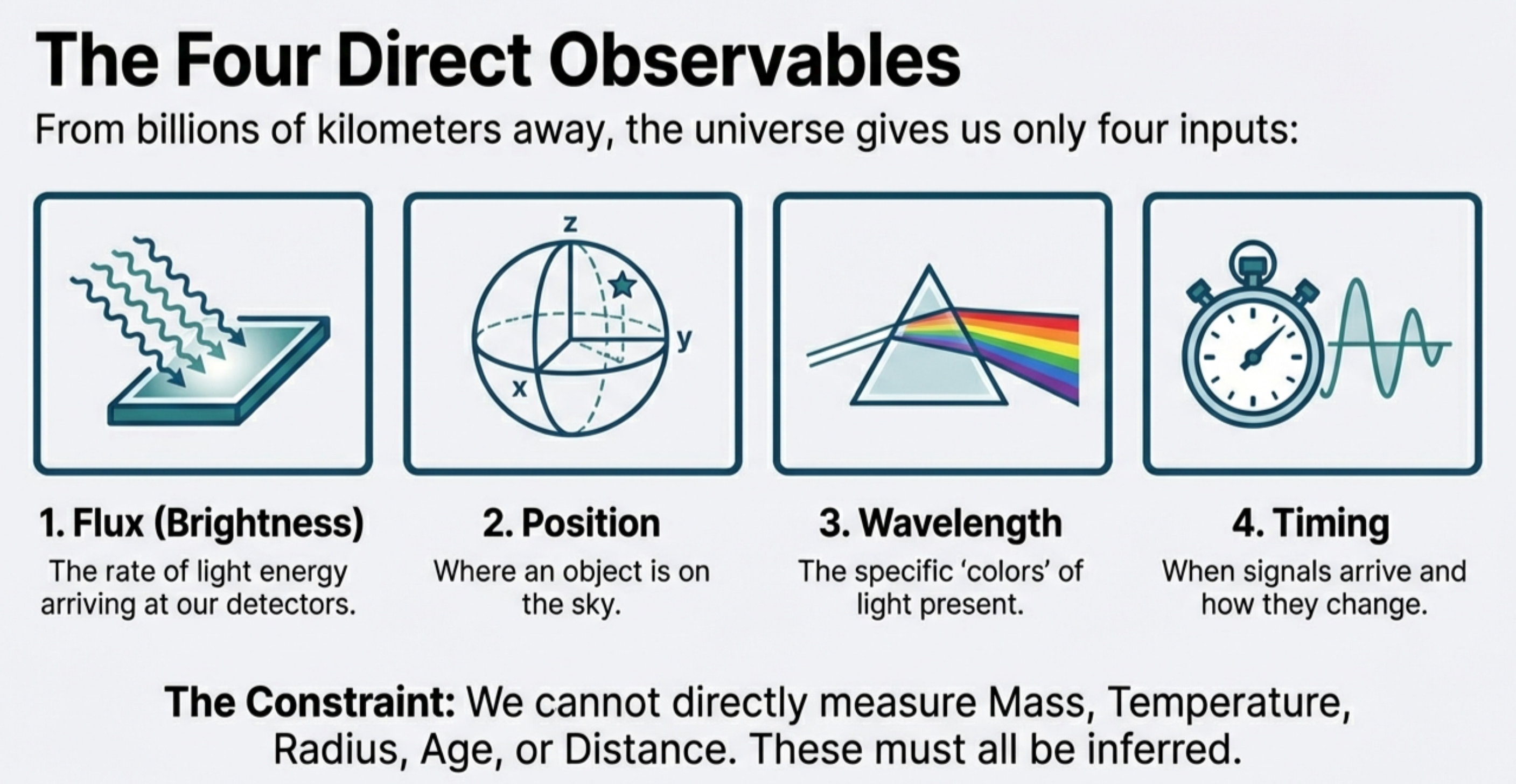
Infographic titled 'The Four Direct Observables' showing four panels: flux (brightness), position, wavelength, and timing, with a note that mass, temperature, radius, age, and distance cannot be directly measured and must be inferred.

What to notice: The universe gives us only four direct inputs: flux, position, wavelength, and timing. Everything else must be inferred. (Credit: (A. Rosen/NotebookLM))

For Lecture 15, two observables matter most:

Position: where the star appears on the sky, and how that position changes over time
Apparent brightness: how much light energy arrives at our detector here on Earth

Those are measurable. But the quantities we actually want are hidden:

Distance: how far away the star really is
Luminosity: how much power the star is actually emitting

That distinction matters. If we blur it, we end up saying things like “that star is bright, so it must be close” or “that star is faint, so it must be weak.” Astronomy gets interesting exactly where those shortcuts fail.

Flowchart titled From Observation to Stellar Physics, showing observables feeding into parallax and inverse-square-law reasoning, then into distance and luminosity, and finally into the H-R diagram.

What to notice: the logic runs in stages. Position change gives parallax, parallax gives distance, brightness plus distance gives luminosity, and luminosity combined with temperature places the star on the H-R diagram.

Apparent brightness: The light energy per unit area per unit time arriving at a detector. This is what we directly measure.

Luminosity: The total power a star emits in all directions. This is an intrinsic property of the star, not a property of our viewpoint.

If a star is moved farther away while everything about the star itself stays the same, should its observed position shift over the year get larger or smaller?

Solution

It should get smaller. More distant stars show smaller parallax shifts, which is why parallax becomes hard to measure for faraway objects.

Now we can state the detective strategy clearly. Use position changes to infer distance. Then use distance plus observed brightness to infer luminosity.

Parallax: Solve Distance First

The Geometry of Nearby Stars

Parallax is the apparent shift in position of a nearby object against a distant background when you observe it from two different vantage points. You can feel the idea in everyday life: hold your finger at arm’s length and alternately close each eye. Your finger appears to jump against the background wall, not because your finger moved, but because you changed position.

For nearby stars, Earth supplies the changing viewpoint. Six months apart, Earth is on opposite sides of its orbit, separated by about 2 AU. That baseline is enormous by human standards and tiny by interstellar standards, which is why the observed stellar shifts are so small.

Geometry diagram of stellar parallax showing Earth at two positions in its orbit, a nearby star above the orbital circle, distant background stars, and sight lines that define a small parallax angle at the star.

What to notice: the nearby star appears to shift only because Earth observes it from opposite sides of its orbit. The parallax angle is half the full swing, and more distant stars make smaller triangles. (Credit: cococubed.com)

Scale comparison chart showing angles in arcseconds for the Full Moon, Jupiter, a typical stellar parallax, and Gaia precision, with bars shrinking dramatically toward the tiny stellar values.

What to notice: stellar parallax is tiny compared with familiar sky angles. The Full Moon spans about 1800 arcseconds, while many stellar parallaxes are hundredths or thousandths of an arcsecond.

The logic is:

Measure the star’s apparent position at one time of year.
Measure it again six months later.
Extract the tiny angular shift relative to very distant background stars.
Use geometry to convert that angle into distance.

Astronomers package this geometry into one beautifully compact rule:

\[ d_{\text{parsec}} = \frac{1}{p_{\text{arcseconds}}} \]

where $d$ is the distance in parsecs and $p$ is the parallax angle in arcseconds.

Parallax angle ($p$): Half the total apparent angular shift of a nearby star as Earth moves from one side of its orbit to the other.

Parsec (pc): The distance at which a star would show a parallax angle of exactly 1 arcsecond. One parsec is about 3.26 light-years.

What makes this so powerful is that it does not depend on a model of stellar physics. We do not need to know what kind of star it is, how hot it is, or how it shines. Parallax is geometry first and astrophysics second.

If a star’s parallax angle is cut in half, what happens to its distance?

Solution

The distance doubles. Since $d = 1/p$, halving $p$ makes $d$ twice as large.

Worked Example: Proxima Centauri

Proxima Centauri, the nearest known star beyond the Sun, has a measured parallax angle of $p = 0.768$ arcseconds.

Distance in parsecs:

\[ d = \frac{1}{0.768} = 1.30 \text{ pc} \]

Convert to light-years:

\[ d = 1.30 \text{ pc} \times 3.26 \frac{\text{ly}}{\text{pc}} = 4.24 \text{ ly} \]

That means the light we see from Proxima tonight left the star more than four years ago.

A star has a parallax angle of 0.1 arcseconds. How far away is it (a) in parsecs and (b) in light-years?

Solution

Using $d = 1/p$: \[ d = \frac{1}{0.1} = 10 \text{ pc} \]
Converting to light-years: \[ d = 10 \text{ pc} \times 3.26 \frac{\text{ly}}{\text{pc}} = 32.6 \text{ ly} \]

The smaller parallax angle means the star is farther away.

🔭 Demo Exploration: Parallax Distance

Use the interactive below to turn the equation into geometric intuition. The goal is not just to get the right number, but to feel how quickly the parallax angle collapses as distance grows.

Open in new tab ↗

Try three quick checks:

Find the setup where the parallax is 0.1 arcseconds. Does the demo agree that the distance is 10 pc?
Halve the distance. What happens to the parallax angle?
Push the star farther away until the shift feels almost invisible. Why does that limit matter for real observatories?

Why Parallax Has Limits

The farther the star, the smaller the angular shift. That is the blessing and the curse of the method. It is direct, but the signal becomes tiny. Ground-based observatories historically struggled below about 0.01 arcseconds, which limited precise parallax measurements to the nearby stellar neighborhood.

Parallax is the first rung of stellar distance measurement because it is the most direct one. It uses geometry, not assumptions about how stars work. But it reaches only as far as our angular precision allows.

Once distance is solved, we can return to the original mystery. A star may still look bright or faint, but now we know how far away it is. That unlocks the second hidden variable.

Brightness vs. Luminosity: Solve the Second Unknown

Here is the central ambiguity again, stated more carefully. A telescope directly measures apparent brightness — the flux of light arriving here. But astronomers often want luminosity — the star’s total power output. Those are not the same quantity.

If two stars have the same luminosity but one is farther away, the farther one looks dimmer. If two stars appear equally bright, one of them might actually be much more luminous if it is also much farther away.

Can a more luminous star appear exactly as bright as a dimmer star?

Solution

Yes. If the more luminous star is also farther away, the extra distance can spread its light over a larger area and cancel the luminosity advantage. Apparent brightness alone does not reveal intrinsic power.

The relationship that connects the observable and the hidden quantity is the inverse-square law:

If a star moves twice as far away, what happens to the light reaching Earth?

A) Half as bright
B) One quarter as bright
C) One eighth as bright

\[ b = \frac{L}{4\pi d^2} \]

where:

$b$ is the apparent brightness (flux) in W/m$^2$
$L$ is the luminosity in watts
$d$ is the distance from the star
$4\pi d^2$ is the area of a sphere centered on the star

Two-panel geometry diagram showing light from a star spreading over a sphere of radius d and then a sphere of radius 2d, with surface areas labeled 4 pi d squared and 16 pi d squared and a note that brightness drops to one fourth.

What to notice: the inverse-square law is geometry, not magic. At twice the distance, the same light must cover four times the area, so the per-area brightness falls to one quarter.

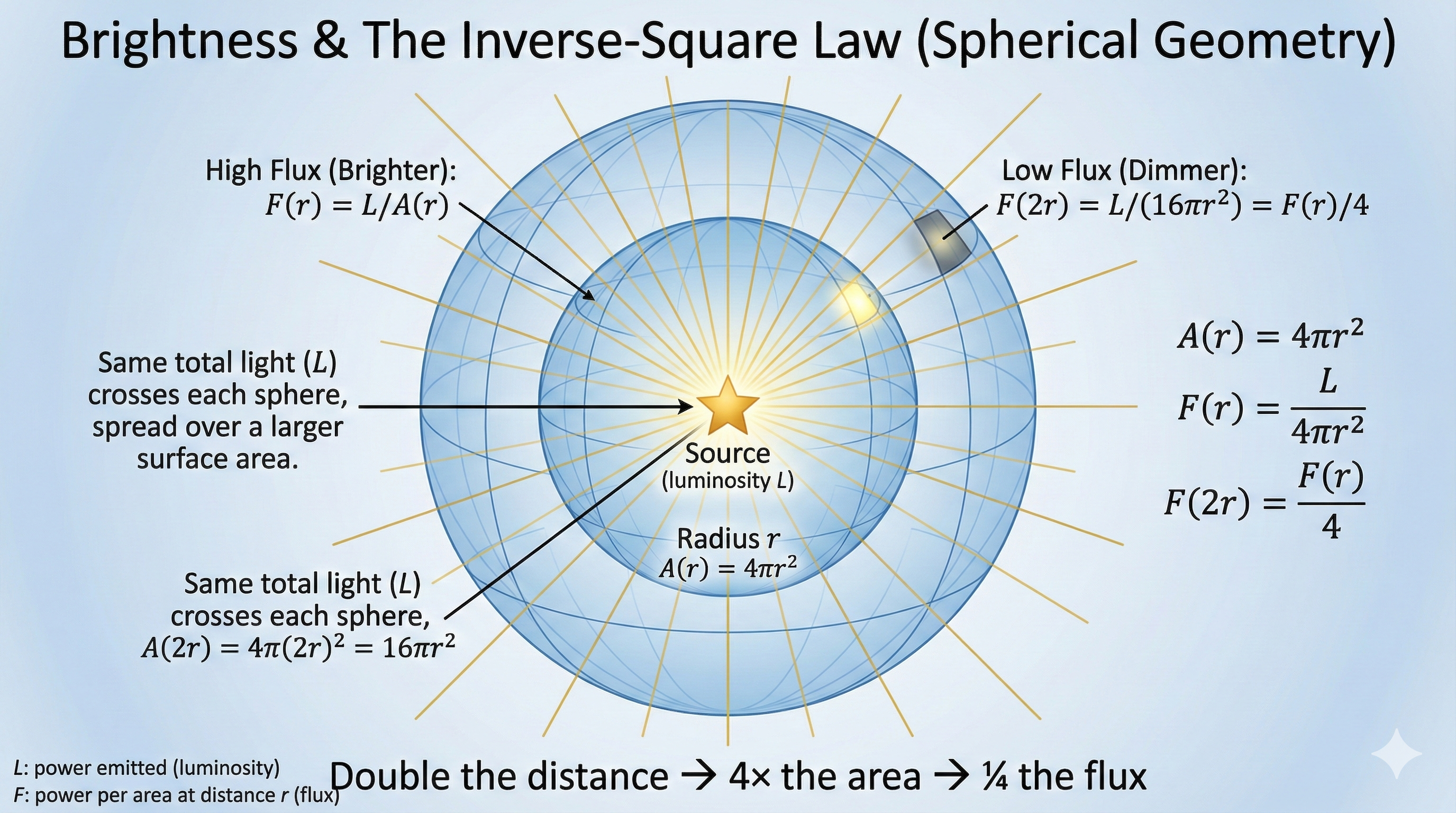
Diagram illustrating the inverse-square law for light: the same total light spreads over larger spherical surfaces at greater distances, reducing intensity.

What to notice: as distance increases, the same light spreads over a larger area, so intensity drops as 1/r². (Credit: (A. Rosen/Gemini))

This equation says something simple and profound: the same total light is being spread over a larger and larger sphere as distance increases. Double the distance and the same energy is spread over four times the area, so the apparent brightness falls by a factor of four.

Prediction Check

The correct answer is B: one quarter as bright. Twice the distance means four times the area, so the same light is diluted by a factor of 4.

Worked Example: Same Apparent Brightness, Different Star

Consider two stars:

Star A: luminosity = 10 $L_\odot$, distance = 10 pc
Star B: luminosity = 40 $L_\odot$, distance = 20 pc

Using the inverse-square law, compare their apparent brightnesses:

\[ b_A \propto \frac{10}{10^2} = \frac{10}{100} = 0.10 \]

\[ b_B \propto \frac{40}{20^2} = \frac{40}{400} = 0.10 \]

They appear equally bright. Star B is four times more luminous, but it is also twice as far away, so its light is spread over four times the area.

That is why the detective strategy has to come in the right order. First solve distance. Then solve luminosity.

Star X appears 4 times brighter than Star Y. Both stars have the same luminosity. Which is closer, and by what factor?

Solution

Using $b \propto 1/d^2$, a factor of 4 in brightness corresponds to a factor of 2 in distance.

So Star X is 2 times closer than Star Y.

A star is measured to have an apparent brightness of $b = 8 \times 10^{-9}$ W/m$^2$ and a parallax angle of $p = 0.05$ arcseconds. Another measurement suggests the star’s luminosity is $L = 100 \, L_\odot$. Are these measurements roughly consistent? (Use $L_\odot = 3.8 \times 10^{26}$ W.)

Solution

From parallax, \[ d = \frac{1}{0.05} = 20 \text{ pc} = 6.17 \times 10^{17} \text{ m} \]

If $L = 100 L_\odot$, then \[ L = 3.8 \times 10^{28} \text{ W} \]

Predict the apparent brightness: \[ b = \frac{L}{4\pi d^2} = \frac{3.8 \times 10^{28}}{4\pi (6.17 \times 10^{17})^2} \approx 7.95 \times 10^{-9} \text{ W/m}^2 \]

That agrees well with the measured value of $8 \times 10^{-9}$ W/m$^2$. So yes, the measurements are roughly consistent.

Magnitude as Astronomical Bookkeeping

Up to this point, the story has been physical and intuitive: angle gives distance, and distance plus flux gives luminosity. Then astronomy hands you one of its least intuitive traditions: magnitudes.

The magnitude system is historical bookkeeping. It survives because astronomers have been using it for centuries, not because it is the cleanest way to think about stellar physics.

Apparent Magnitude

Apparent magnitude $m$ is a logarithmic way to record how bright a star appears from Earth. The awkward part is that the scale runs backward: smaller numbers mean brighter objects.

\[ m_1 - m_2 = -2.5 \log_{10}\left(\frac{b_1}{b_2}\right) \]

So a 5-magnitude difference corresponds to a factor of 100 in brightness.

Two-panel infographic with a table converting magnitude differences to brightness ratios and a simple distance-modulus visual comparing a star at 10 parsecs to the same star farther away, labeled with M, m, and m minus M.

What to notice: two useful translation rules tame the magnitude system. A difference of 5 magnitudes means a factor of 100 in brightness, and the distance modulus compares how bright a star looks now to how bright it would look at 10 pc.

Apparent magnitude ($m$): A logarithmic brightness scale measured from Earth. Brighter objects have smaller magnitude numbers.

If astronomers had invented a fully intuitive brightness scale from scratch, would you expect a larger number to mean brighter or dimmer? What does the actual magnitude system do instead?

Solution

Most people would expect a larger number to mean brighter. But the actual magnitude system is historical and reversed: larger magnitude numbers mean dimmer objects.

For example:

the Sun has apparent magnitude $m = -26.8$
Sirius has $m = -1.46$
the faintest naked-eye stars are around $m = 6$

Absolute Magnitude

To compare stars fairly, astronomers define absolute magnitude $M$: the apparent magnitude a star would have if it were placed at exactly 10 parsecs away.

That lets magnitudes do the same job luminosity does, but in the older notation system. If two stars are placed at the same standard distance, the brighter one intrinsically will have the smaller absolute magnitude.

Absolute magnitude ($M$): The apparent magnitude a star would have if it were placed at a standard distance of 10 parsecs.

Distance Modulus: The Translation Rule

The standard relation connecting apparent magnitude, absolute magnitude, and distance is the distance modulus:

\[ m - M = 5\log_{10}(d) - 5 \]

where $d$ is in parsecs.

Conceptually, this is just the inverse-square law written in magnitude language. The bigger the difference between how bright a star looks and how bright it would look at 10 pc, the farther away it must be.

What magnitude difference corresponds to a factor of 100 in brightness?

Solution

Five magnitudes. That is the key conversion worth memorizing.

Worked Example: Reading a Distance Modulus

Suppose a star has apparent magnitude $m = 10$ and absolute magnitude $M = 5$. Then:

\[ m - M = 10 - 5 = 5 \]

Use the distance modulus:

\[ 5 = 5\log_{10}(d) - 5 \]

\[ 10 = 5\log_{10}(d) \]

\[ 2 = \log_{10}(d) \]

\[ d = 10^2 = 100 \text{ pc} \]

The star appears 5 magnitudes dimmer than it would at 10 parsecs, so it must be farther away. The distance modulus turns that brightness difference back into a distance estimate.

If a star has $m = 8$ and $M = 3$, what distance modulus does it have, and does that mean the star is closer than 10 pc, exactly 10 pc, or farther than 10 pc?

Solution

The distance modulus is \[ m - M = 8 - 3 = 5 \]

A positive distance modulus means the star appears dimmer than it would at 10 pc, so it must be farther than 10 parsecs. In fact, a modulus of 5 corresponds to 100 pc.

The magnitude system feels strange because it preserves ancient observational habits inside modern quantitative astronomy.

Hipparchus ranked stars visually long before astronomers had physical units for energy flux. Nineteenth-century astronomers later formalized the system mathematically but preserved the old direction of the scale. Today magnitudes are useful because they are standard and compact, but for conceptual understanding it is usually better to think in luminosity, flux, and distance first.

The Distance Ladder

Parallax is powerful, but it does not reach everywhere. The angles simply become too small. That is why astronomy uses a distance ladder: a sequence of methods that build outward from the geometric anchor provided by parallax.

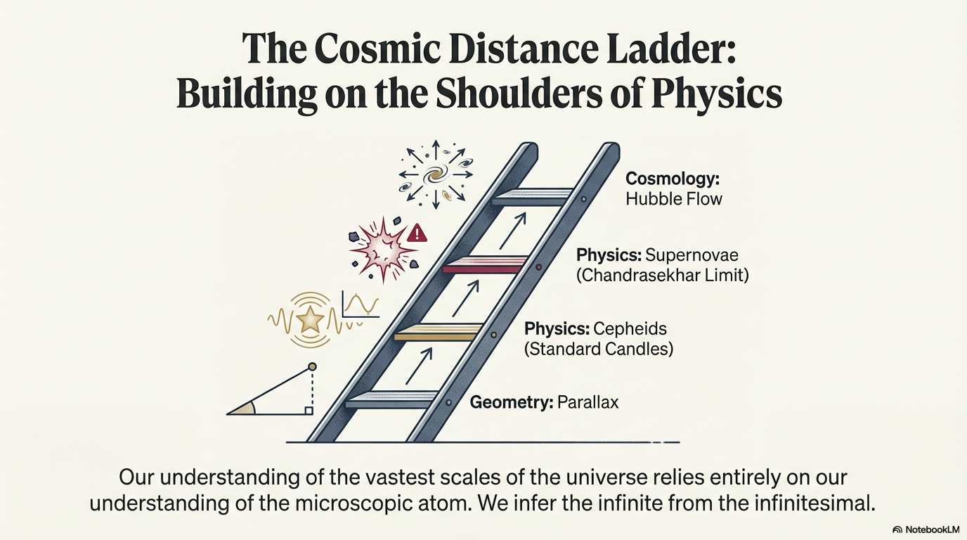
Four-rung ladder diagram titled 'The Cosmic Distance Ladder: Building on the Shoulders of Physics'. From bottom to top: Rung 1 Geometry (Parallax), Rung 2 Physics (Cepheids/Standard Candles), Rung 3 Physics (Supernovae/Chandrasekhar Limit), Rung 4 Cosmology (Hubble Flow). Footer text: Our understanding of the vastest scales relies on the microscopic atom.

What to notice: Each rung calibrates the next. Parallax (geometry) → Cepheids (standard candles) → Supernovae (Chandrasekhar limit) → Hubble Flow (cosmology). We infer the infinite from the infinitesimal. (Credit: (A. Rosen/NotebookLM))

The logic of the ladder is not “one method failed, so try another random one.” The logic is calibration.

Parallax gives direct nearby distances from geometry.
Those distances calibrate standard candles such as Cepheids.
Standard candles calibrate more distant tools, including Type Ia supernovae.
At the largest scales, cosmology uses the expansion of the universe itself.

Each rung reaches farther, but each one depends on the reliability of the rung below it.

Why can’t geometry alone carry us all the way to distant galaxies?

Solution

Because the parallax angles become far too small to measure. The method itself is still valid, but the signal shrinks beyond practical precision. To go farther, astronomers need new observables whose intrinsic properties can be calibrated from nearby objects.

This is what makes parallax the first rung rather than just one method among many. It anchors the whole system.

Gaia and Why Precision Matters

The history of stellar distance measurement is really the history of getting better at measuring absurdly tiny angles.

Ground-based astronomy could reach parallax precisions of roughly 0.01 arcseconds, which limited reliable distances to the nearby stellar neighborhood. Hipparcos pushed that to roughly 0.001 arcseconds from space and transformed nearby-star astronomy. Gaia pushed much farther still.

Gaia, launched by the European Space Agency in 2013, measures parallaxes for billions of stars and can reach precisions of order 10 microarcseconds for its best targets. That does not mean every star in the sky gets that precision, but it does mean the Milky Way can now be mapped in three dimensions with a level of detail that earlier generations of astronomers could barely imagine.

$Milky Way context diagram showing the Sun's location in the disk, a smaller nearby neighborhood, and a much larger Gaia reach region extending across a substantial fraction of the galaxy.$

What to notice: Gaia does not merely improve one nearby distance here or there. Its parallax reach extends across a large fraction of the Milky Way, turning local geometry into a three-dimensional galactic map.

If Gaia can measure a parallax as small as 10 microarcseconds for an exceptionally favorable target, what distance does that correspond to?

Solution

Convert 10 microarcseconds to arcseconds: \[ 10 \, \mu\text{as} = 10 \times 10^{-6} \text{ arcseconds} = 10^{-5} \text{ arcseconds} \]

Then use $d = 1/p$: \[ d = \frac{1}{10^{-5}} = 100{,}000 \text{ pc} \]

That is about 326,000 light-years. So in the best cases, Gaia can reach across the Milky Way and into the nearest galactic neighborhood, but not to Andromeda as a whole.

Gaia matters because it sharpens everything downstream. Better distances mean better luminosities. Better luminosities mean cleaner H-R diagrams. Cleaner H-R diagrams mean more trustworthy stellar ages, radii, and evolutionary stories. Precision in one foundational measurement propagates through the whole of stellar astrophysics.

Even the nearest stars are so far away that Earth’s orbit becomes a tiny geometric baseline.

That is the humbling part of stellar astronomy. Earth’s orbit feels enormous in daily life, but against interstellar distances it is almost nothing. The fact that a simple geometric trick still works is one of the triumphs of careful measurement.

Synthesis: First Distance, Then Luminosity

By now the detective chain should feel straightforward:

Measure changing position -> determine parallax
Convert parallax into distance
Measure arriving flux -> determine apparent brightness
Apply the inverse-square law -> determine luminosity
Combine luminosity with temperature -> place the star on the H-R diagram

Once distance and luminosity are known, the rest of stellar astronomy opens up. We can combine luminosity with temperature to infer radius. We can place the star on the H-R diagram. Later, binary orbits will let us add mass, and then the full architecture of stellar lives comes into view.

Two stars appear equally bright.

Star A: distance = 10 pc
Star B: distance = 100 pc

Which star is more luminous?

Solution

Star B is more luminous. It is 10 times farther away, so to appear equally bright it must emit $10^2 = 100$ times more total power.

Common Misconceptions

“Brighter-looking stars are always closer”

Not true. A bright star might be nearby, intrinsically luminous, or both. Brightness alone does not separate those possibilities. That is exactly why Lecture 15 exists.

“Parallax is just another model”

Not in the same sense as stellar evolution or standard candles. Parallax is geometric. It is the cleanest direct method we have because it does not depend on assumptions about how stars shine.

“Magnitudes tell me more physics than luminosity does”

No. Magnitudes are useful notation, but they are still notation. The underlying physics is in flux, luminosity, distance, and the inverse-square law.

“Stars at the same distance should look equally bright”

Only if they also have the same luminosity. Equal distance removes one variable, but intrinsic stellar power can still differ enormously.

Summary: First Distance, Then Luminosity

Observable

We directly measure only two crucial clues here: a star’s changing position and the brightness of its light.

Model

Geometry turns parallax into distance. The inverse-square law turns brightness plus distance into luminosity. The magnitude system is the historical shorthand layered on top of the same physics.

Inference

A bright-looking star is not enough. First solve distance, then solve luminosity, and only then can the star be placed meaningfully on the H-R diagram and folded into the wider story of stellar structure.

Looking Ahead

Next lecture, those distances and luminosities become coordinates on the Hertzsprung-Russell diagram. Without Lecture 15, the H-R diagram would be unreadable. With it, temperature and luminosity suddenly organize stars into a pattern. Soon after, binary systems will add mass, and the three great hidden quantities of stellar astronomy — distance, luminosity, and mass — will start to lock together.

Practice Problems

Solutions are available in the Lecture 15 Solutions.

Core Problems (Master these before the exam)

Problem 1: Parallax and Distance

The star Betelgeuse has a measured parallax angle of 4.51 milliarcseconds. Calculate its distance (a) in parsecs and (b) in light-years. (Note: 1 milliarcsecond = 0.001 arcsecond)

Problem 2: Inverse-Square Law

Two stars have the same luminosity (L = $100 \L_\odot$). Star A is at distance 10 pc, Star B is at distance 20 pc. What is the ratio of their apparent brightnesses?

Problem 3: Magnitude Differences

Two stars have apparent magnitudes $m_1 = 1.5$ and $m_2 = 6.5$. How many times brighter (in terms of flux) is Star 1 than Star 2?

Problem 4: Luminosity from Distance and Brightness

A star has an apparent brightness of $b = 5 \times 10^{-12}$ $W/m^{2}$ and a parallax angle of 0.2 arcseconds. Calculate its luminosity in watts and in units of solar luminosities.

Problem 5: Distance Modulus

A Cepheid variable star has absolute magnitude $M = -3.5$ and apparent magnitude $m = 13.5$. Use the distance modulus ($m - M = 5 \log_{10}(d) - 5$) to find its distance in parsecs and kiloparsecs.

Challenge Problems (Stretch your thinking)

Challenge 1: The Distance Ladder

You discover a new Type Ia supernova in a distant galaxy. Type Ia supernovae have a known absolute magnitude at peak brightness of $M = -19.3$. You measure the supernova’s apparent magnitude to be $m = 19.3$.

Use the distance modulus to calculate the distance in megaparsecs.
How many times more distant is this galaxy than Andromeda (770 kpc)?

Challenge 2: Gaia’s Precision

Gaia measures the parallax angle of an exceptionally favorable target to be $p = 10.0 \pm 0.5$ microarcseconds. What is the distance (a) in parsecs and (b) in light-years? What is the fractional uncertainty in the distance?

Challenge 3: An Unseen Companion

A star has an apparent brightness $b = 1 \times 10^{-11}$ $W/m^{2}$ and distance 20 pc (measured via parallax). Its calculated luminosity is $2 \L_\odot$. But if you measure the star’s spectrum carefully, you discover it is only about $1 \L_\odot$ bright. The discrepancy suggests the star has an unseen companion. What is the luminosity of the companion?

Glossary

★ Absolute magnitude: Apparent magnitude at standard distance of 10 pc Symbol: $M$; Units/context: dimensionless
★ Apparent brightness: Flux of light energy arriving at Earth from a star Symbol: $b$; Units/context: W/m²
★ Apparent magnitude: Historical brightness scale (brighter = smaller number) Symbol: $m$; Units/context: dimensionless
★ Distance ladder: Sequence of methods for measuring cosmic distances Units/context: conceptual
★ Distance modulus: Relationship between apparent magnitude, absolute magnitude, and distance Symbol: $m - M$; Units/context: dimensionless
★ Gaia: European space mission for precise parallax measurement Units/context: proper noun
★ Inverse-square law: Flux decreases with distance squared Symbol: $b = L / 4\pi d^2$
★ Light-year: Distance light travels in one year Symbol: ly; Units/context: 9.46 × 10¹⁵ m
★ Luminosity: Total power radiated by a star in all directions Symbol: $L$; Units/context: W (watts)
★ Parallax angle: Half the total angular shift in a star's position over 6 months Symbol: $p$; Units/context: arcseconds (″)
★ Parsec: Distance unit: distance at which parallax angle = 1 arcsecond Symbol: pc; Units/context: 3.086 × 10¹⁶ m
★ Solar luminosity: The Sun's luminosity; standard reference Symbol: L☉; Units/context: 3.8 × 10²⁶ W
★ Spectral type: Classification of stars by temperature (OBAFGKM) Units/context: categorical