Lecture 22: The Milky Way and the First Hidden Thing
Our Galactic Home and the Case for Dark Matter
The Big Idea
Our galaxy is a rotating stellar system whose visible stars do not contain enough mass to hold it together. The flatness of its rotation curve — measured with the light of stars and hydrogen gas — forces us to conclude that most of the Milky Way is made of something we cannot see directly. That something is the first of Module 3’s three hidden things.
Observable: Stars and neutral hydrogen orbit the Milky Way at roughly constant speed far from the center.
Model: Circular orbits in a gravitational potential connect speed and enclosed mass through \(M_{\text{enc}} = v^2 r/G\).
Inference: The enclosed mass keeps growing beyond the visible disk, so the galaxy contains a large halo of non-luminous matter.
Main uncertainty: The rotation curve tells us that extra gravity is present; it does not, by itself, identify the particle or prove which microscopic substance causes the extra gravity.
This page answers three questions:
- What does the Milky Way actually look like, and how do we know?
- How do we weigh a galaxy when most of its mass emits no light?
- What sits at the center of our galaxy, and how do we know its mass?
Punchline: A galaxy’s rotation curve is a stellar-kinematics measurement that demands dark matter, and the stars near Sgr A* are a stellar-kinematics measurement that demands a supermassive black hole.
Our Milky Way galaxy is home to more than 100 billion stars that are often separated by trillions of miles. The spaces in between, called the interstellar medium, are not empty; they are sprinkled with gas and dust that are both the seeds of new stars and the leftover crumbs from stars long dead. Studying the interstellar medium with observatories like NASA’s upcoming Nancy Grace Roman Space Telescope will reveal new insight into the galactic dust recycling system.
This reading moves from the Milky Way’s visible structure to the invisible mass that holds it together, and closes with the supermassive black hole at its center.
Default expectation (best): Read the whole page before lecture and stop at each Check Yourself prompt.
If you’re short on time (~20 min): Focus on:
- The Big Idea above
- Structure of the Milky Way (the four main components)
- The Rotation Curve section (the central argument for dark matter)
- Sagittarius A* (the worked example using Kepler’s third law)
Goal after 20 minutes: You should be able to describe what dark matter is and is not, explain how we infer its presence from observation, and describe the evidence for a supermassive black hole at the Galactic Center.
Reference mode: Use the Structure Reference Box, the Rotation Curve figure, and the Glossary as a study reference through the rest of Module 3.

What to notice: Module 3 uses the same evidence chain over and over. Dust, 21-cm emission, S-star orbits, galaxy shapes, Cepheid periods, supernova brightness, redshifts, AGN jets, CMB anisotropies, and light-element abundances become physical claims only after a model translates them. (Credit: Illustration: A. Rosen (SVG))
Learning Outcomes
By the end of this reading, you should be able to say:
Where We Live
Step outside on a dark, moonless night, far from city lights, and look up. A faint band of diffuse light arches across the sky. That band has a name — the Milky Way — and it has a physical meaning that ancient observers could not have guessed.
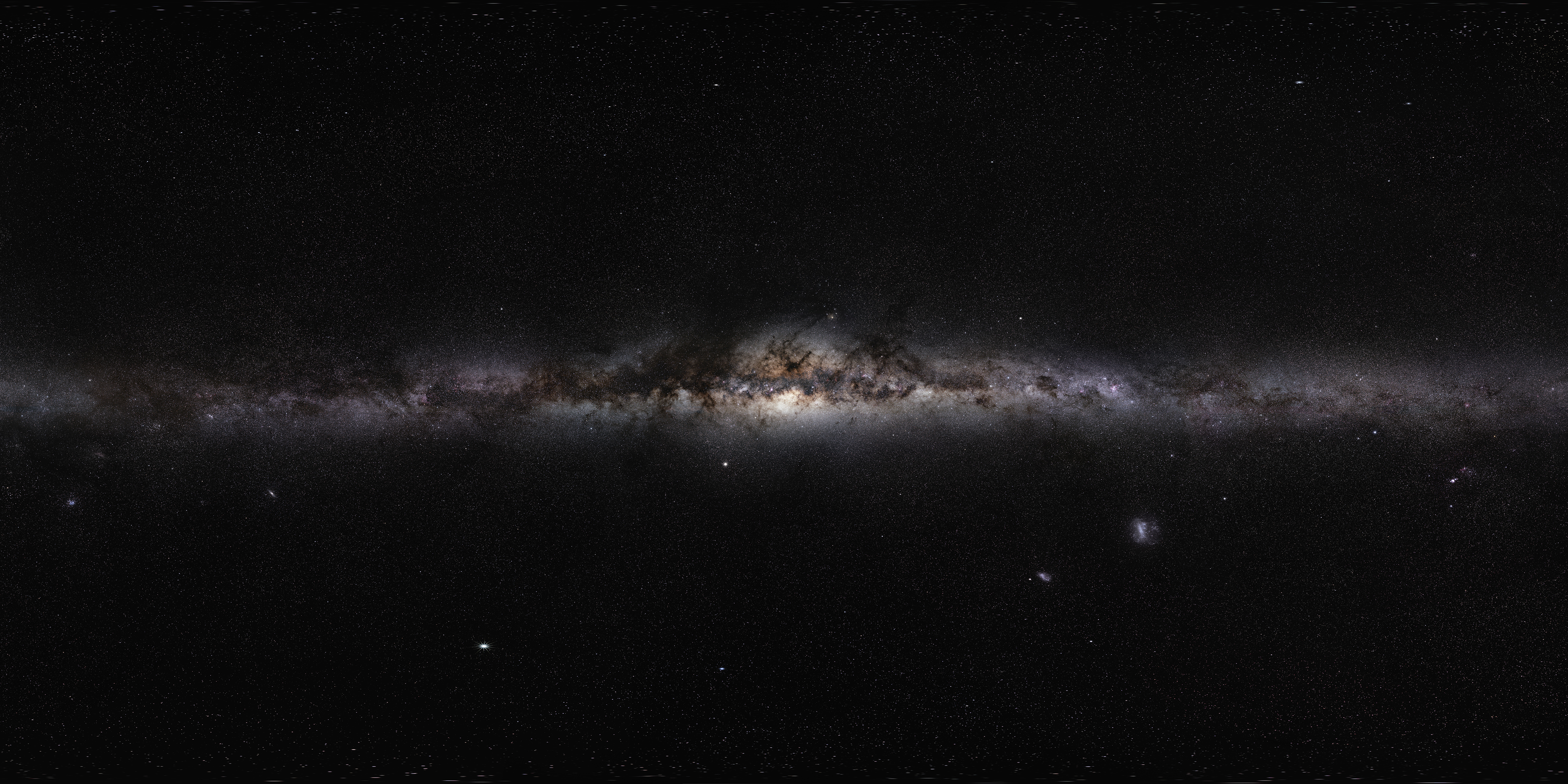
What to notice: even a ‘pretty picture’ is a measurement—brightness and color patterns carry physical information.
That band is unresolved starlight, seen edge-on through our own galaxy. We are not looking at the Milky Way from the outside. We are looking along it from the inside. Everything you can see with the unaided eye — every named star, every constellation, the Sun itself — lies within this one galaxy.
The question for today is: what does this galaxy actually look like, and what is it made of? The answers come from stars. Every time we map the Milky Way, it is because stars (and the gas around stars) are telling us something about where they live and how they move.
We live inside the Milky Way and must infer its structure by looking outward from within it.
Structure: The Milky Way in Four Pieces
Imagine you could fly far above the Milky Way and look down. What you would see is a barred spiral galaxy with four distinguishable components:
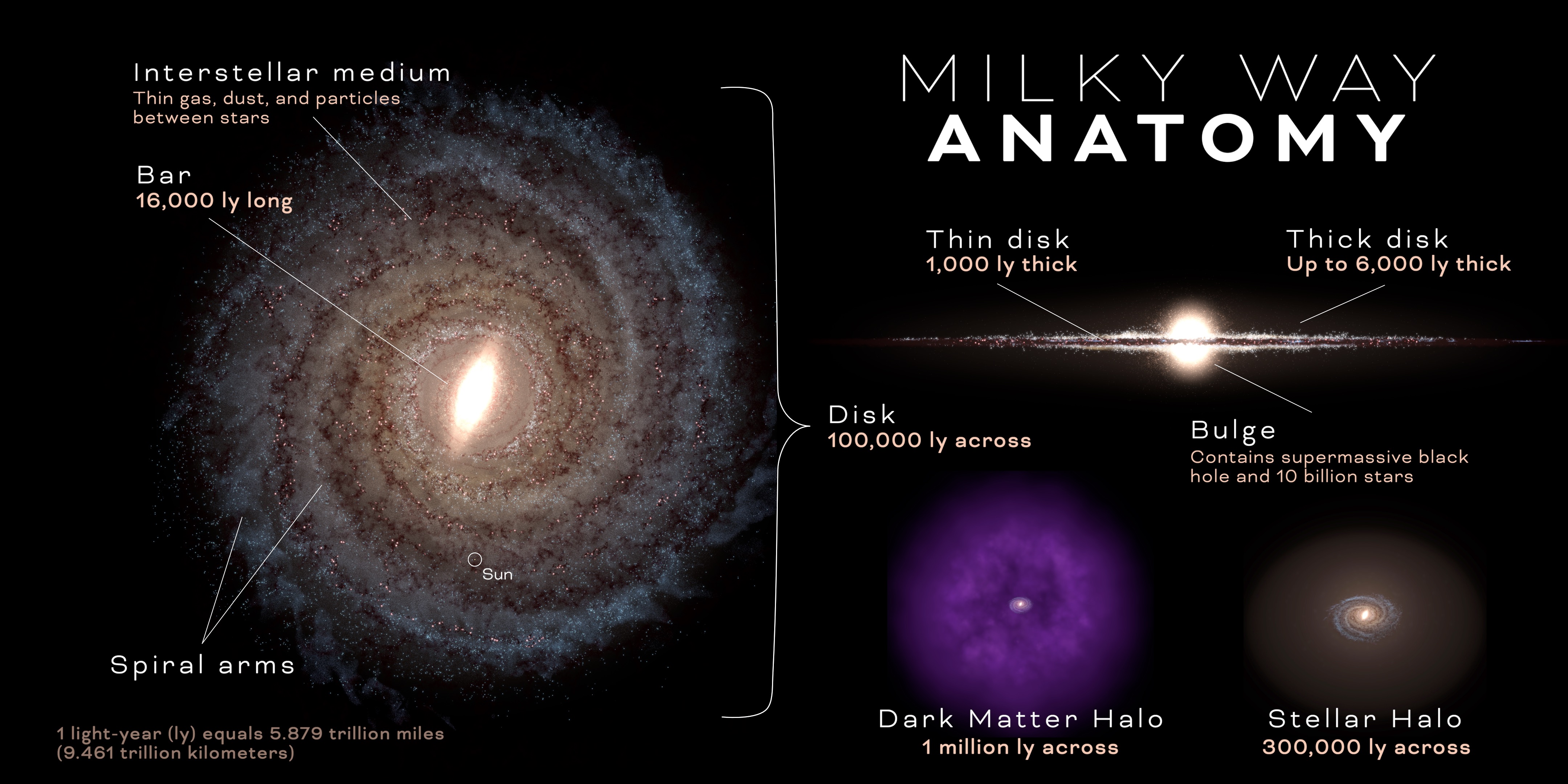
What to notice: the Milky Way is not just a flat spiral disk. It has a thin disk, thick disk, central bar and bulge, spiral arms, interstellar medium, stellar halo, and extended dark-matter halo. (Credit: Course illustration)
Real galactic disks are not rigid plates. Gas can warp, dust lanes can trace tilted structures, and the outer disk responds to the gravity of companions and the surrounding dark-matter halo.
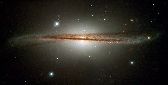
What to notice: galactic disks are not perfectly flat plates. Dust lanes, warps, and tilted outer gas layers show that a galaxy is a dynamical system shaped by gravity, accretion, and interactions. (Credit: Course-provided figure)
1. The Disk. A thin, rotating pancake of stars and gas, ~30 kpc across and only ~0.3 kpc thick. The disk hosts most of the galaxy’s young and intermediate-age stars and almost all of its star-forming gas. The Sun lives in the disk, about 8 kpc from the center.
2. The Bulge and Bar. A denser, roughly ellipsoidal concentration of stars at the center of the disk. In the Milky Way specifically, this central region is elongated into a bar that rotates with the disk. Stars in the bulge are typically older than disk stars.
3. The Stellar Halo. A sparse, roughly spherical distribution of very old stars and globular clusters that surrounds the disk and bulge. Halo stars were born early in the galaxy’s history and have been orbiting on elongated, randomly oriented paths ever since.
4. The Spiral Arms. Bright, wound patterns within the disk traced by young, hot O- and B-type stars (callback to Lecture 16) and by the glowing gas of H II regions where those stars were recently born. Spiral arms are not fixed lanes of material; they are density waves that stars and gas flow through.
The visible disk is only the beginning of the Milky Way’s gravitational footprint. Faint companion galaxies orbit far outside the bright spiral structure, and they are part of the same story as the stellar halo: small systems are continually being pulled into, stretched by, and sometimes absorbed by the larger Galaxy.
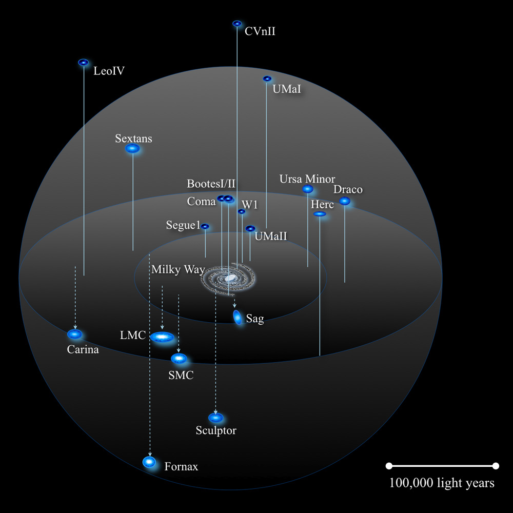
What to notice: the Milky Way is surrounded by faint satellite galaxies, not just by isolated stars. These companions help trace the Galaxy’s larger gravitational environment and its extended dark-matter halo. (Credit: Course-provided figure)
Populations: Reading the Galaxy with Stellar Physics
One of the major payoffs of Module 2 is that each of these four components has a recognizable stellar population. Young blue disk stars, old red halo stars, and intermediate-age bulge stars tell different parts of the Milky Way’s history.
If you know the H-R diagram (Lecture 16) and you know how stellar lifetimes depend on mass (Lecture 19), you can already say things like: the halo must be ancient, because nobody hot and massive lives there anymore. This is not a speculation; it is a direct inference from stellar physics applied to a population of stars.
Globular cluster: A densely packed, roughly spherical collection of 10⁴ – 10⁶ stars bound by their mutual gravity. Globulars are among the oldest structures in the Milky Way, with ages of ~10 – 13 Gyr.
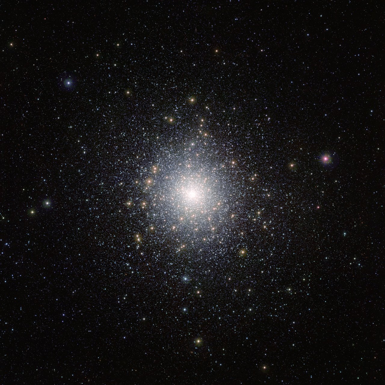
What to notice: a globular cluster is not a loose patch of random stars. It is a dense, old, gravitationally bound stellar population, exactly the kind of object that helps trace the Milky Way’s halo. (Credit: ESO/M.-R. Cioni/VISTA Magellanic Cloud survey)
Modern surveys keep finding faint companions around the Milky Way, especially in the halo. That matters because dwarf galaxies and globular clusters are not just “extra objects.” They are dynamical tracers. Their positions and motions help astronomers map the mass distribution of the Milky Way far beyond the region where the disk’s stars dominate the light.
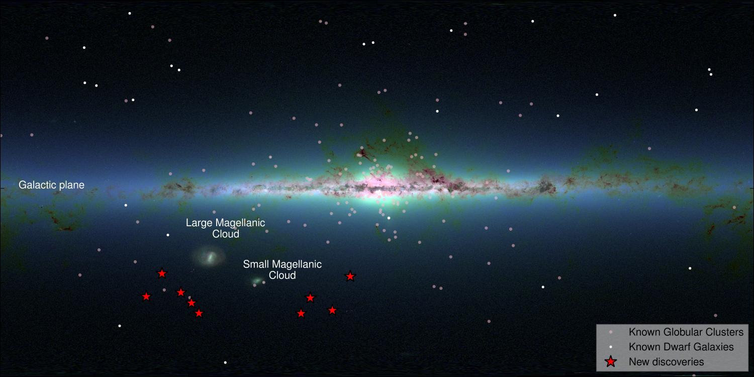
What to notice: the Milky Way’s halo is still being mapped. Known dwarf galaxies, globular clusters, and newly identified faint companions show that the Galaxy’s environment extends far beyond the bright disk. (Credit: Course-provided figure)
Two stars have identical spectra consistent with a K5 dwarf. One orbits in the thin disk on a nearly circular path; the other orbits in the halo on a highly elongated, tilted path. Which was more likely born recently, and which was likely born in the galaxy’s first few billion years?
The disk star is more likely to be younger; the halo star is more likely to be ancient. This is a kinematic inference that rests on how the Milky Way built itself: the disk is where ongoing star formation happens (gas is still there), and its stars inherit the disk’s orderly, near-circular orbits. The halo formed early from accreted material and early collapse; its stars are old and their orbits retained the disorderly motions of that era. Stellar spectral type alone (K5) does not tell you an age — but kinematics plus location does.
The Milky Way has four main components — disk, bulge/bar, halo, and spiral arms — and each hosts a characteristic population of stars that records a different chapter of galactic history.
Mapping a Galaxy You Live Inside
How do you map the inside of something you cannot leave? With two great advantages: the speed of light lets you see billions of stars at once, and the physics of different wavelengths gets around the biggest obstacle — dust.
The Dust Problem
The Milky Way’s disk contains interstellar dust: micron-sized grains that absorb and scatter visible light. Toward the Galactic Center, the dust is so dense that no visible light from the center reaches us. Early-20th-century astronomers did not know this, which is why they initially thought the Sun was near the middle of our Galaxy. It isn’t.
Before comparing the wavelength views below, predict which kind of light is most useful for each target:
- stars hidden behind dust,
- neutral hydrogen gas,
- hot or high-energy structures near the Galactic Center.
Then check whether the figures support your prediction.
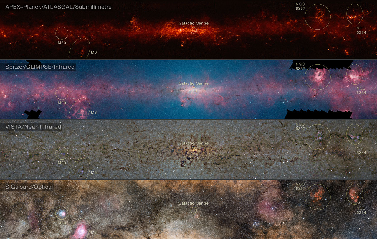
What to notice: the same Galactic Center looks almost opaque in visible light but becomes richly structured at infrared and submillimeter wavelengths. Changing wavelength changes which physical component you can see. (Credit: ESO/ATLASGAL consortium/NASA/GLIMPSE consortium/VVV Survey/ESA/Planck/D. Minniti/S. Guisard)
What to notice: the Galactic Center is crowded, dusty, and multiwavelength by necessity. Near-infrared and high-energy views turn an apparently hidden region into a map of stars, gas, and compact sources. (Credit: Course-provided figure)
Dust is a problem for visible light specifically because visible wavelengths (~0.5 μm) are comparable to the size of dust grains. At longer wavelengths, the grains are less effective at blocking light. This means the solution is to change the wavelength we observe at. In practice, “mapping the Milky Way” always begins with the question: what tracer can get through the material between us and the part of the Galaxy we want to study?
The 21-cm Line: Hydrogen as Our Native Guide
Neutral hydrogen in the interstellar medium can emit a faint but characteristic photon at a wavelength of 21 cm — in the radio part of the spectrum (callback to Lecture 7). This emission comes from a quantum-mechanical transition: the “hyperfine” flip of the electron’s spin relative to the proton’s spin. Any one hydrogen atom emits this photon only rarely, but the Galaxy contains so much neutral hydrogen that the combined signal is detectable and map-like.
At 21 cm, dust is utterly transparent. The galaxy’s HI gas lights up like a map of itself.
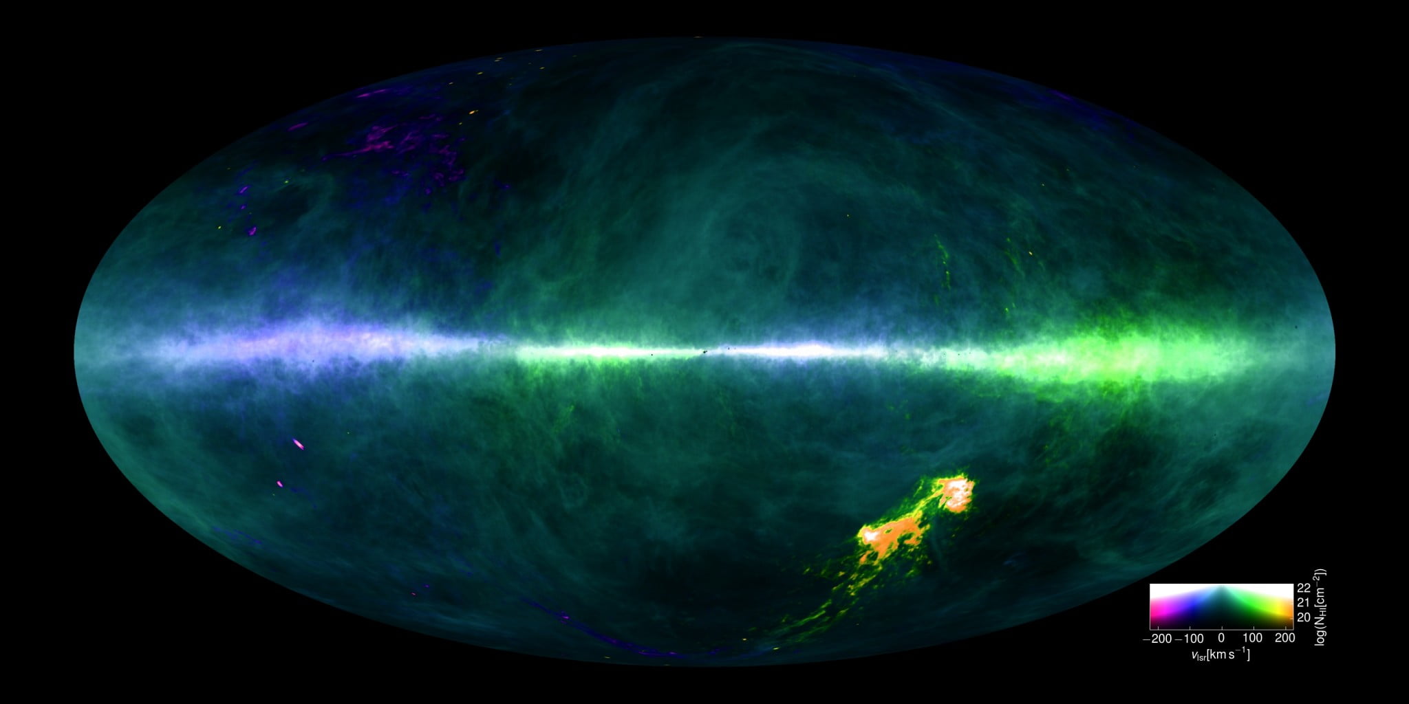
What to notice: 21-cm radio emission turns neutral hydrogen into an all-sky map. The bright band is the Milky Way’s gas-rich disk, and the colors encode velocity information as well as column density. (Credit: Benjamin Winkel and the HI4PI Collaboration)
Radio astronomy is not limited to the 21-cm hydrogen line. Continuum maps can trace ionized gas, energetic particles, and feedback structures around star-forming regions. The point is the same: when visible light is incomplete, changing the wavelength changes the physical question we can ask.
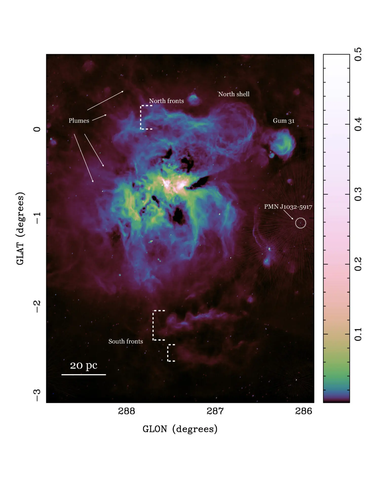
What to notice: radio maps reveal gas structures that optical light can miss or confuse. In the Carina region, shells, fronts, and plumes trace how massive stars reshape the surrounding interstellar medium. (Credit: Course-provided figure)
Even better: because HI is moving, we can Doppler-shift the 21-cm line (callback to Lecture 10) to measure its velocity along our line of sight. This gives us a three-dimensional kinematic map of the Milky Way’s neutral hydrogen, including the parts of the disk hidden behind dust from our position.
Infrared: Seeing Through Dust with Thermal Light
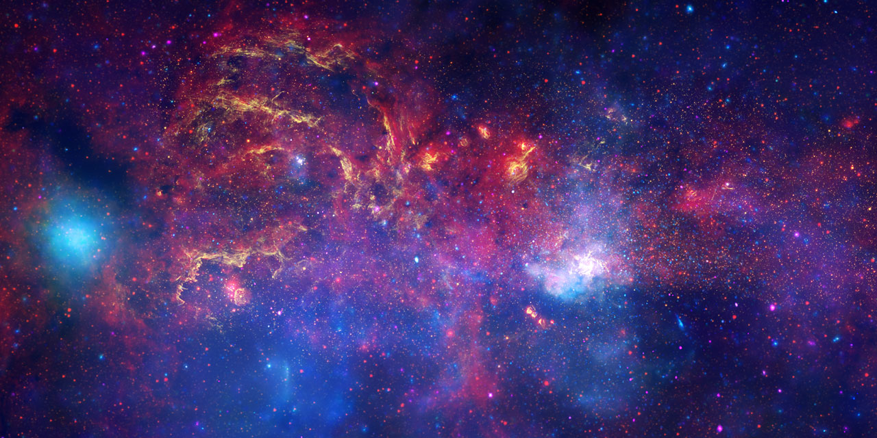
Infrared photons also pass through dust far more easily than visible ones. The Spitzer Space Telescope and, more recently, JWST have revealed the Galactic Center’s dense stellar cluster in detail that optical images cannot achieve. Infrared is how we see the stars behind the dust; 21-cm is how we see the gas behind the dust.
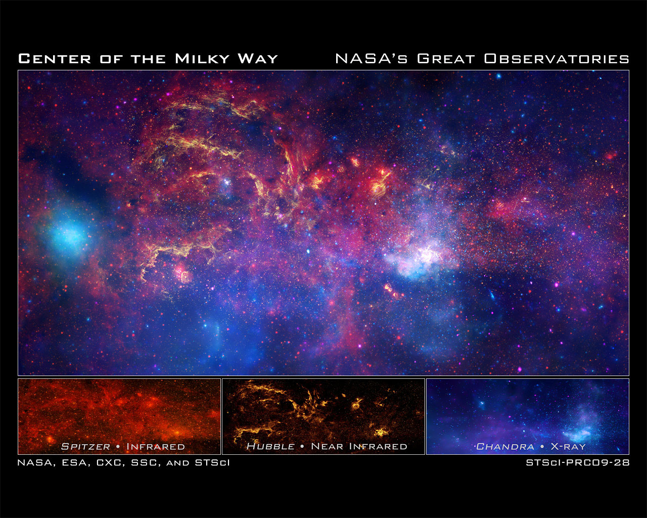
What to notice: the Galactic Center is not one picture. Spitzer infrared, Hubble near-infrared, and Chandra X-ray observations reveal dust, stars, hot gas, and compact high-energy sources in the same crowded region. (Credit: NASA, ESA, SSC, CXC, and STScI)
The same logic works in nearby star-forming regions. A dusty nebula can look confusing or opaque in visible light, but infrared light turns the dust and embedded young stars into a readable map of where star formation is happening.
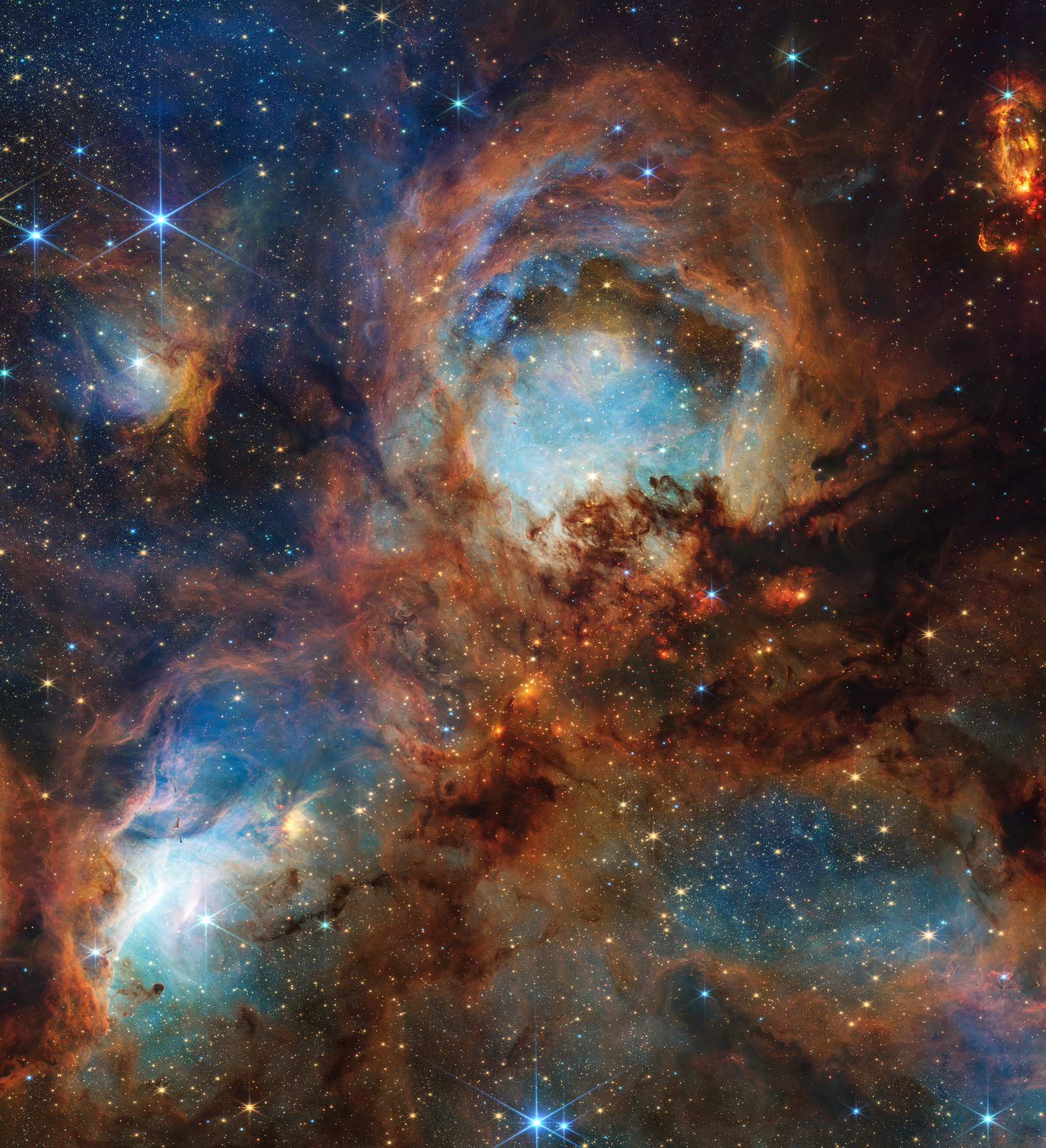
What to notice: infrared light turns dusty star-forming gas from an obstacle into evidence. The same dust that hides visible light can outline where new stars are forming. (Credit: Course-provided figure)

What to notice: Gaia does not merely improve one nearby distance here or there. Its parallax reach extends across a large fraction of the Milky Way, turning local geometry into a three-dimensional galactic map.
Gaia, by contrast, works at visible wavelengths and measures precise stellar parallaxes (callback to Lecture 15). It cannot see through dust toward the Galactic Center, but within the parts of the disk it can reach, it has measured the three-dimensional positions and velocities of well over a billion stars — a transformational dataset that has, for example, revealed the imprint of past minor mergers in the stellar halo.
As you watch, keep the evidence chain in mind: Gaia measures positions, parallaxes, and motions for individual stars; the map appears only after those measurements are stitched together into a model of the Galaxy.
Source: ESA, The best Milky Way animation, by Gaia. Credit: ESA/Gaia/DPAC, Stefan Payne-Wardenaar.
There is one more clever mapping trick: use objects behind the Milky Way as flashlights. A distant quasar can shine through gas in our halo, and absorption lines in the quasar spectrum reveal gas that would otherwise be nearly invisible.
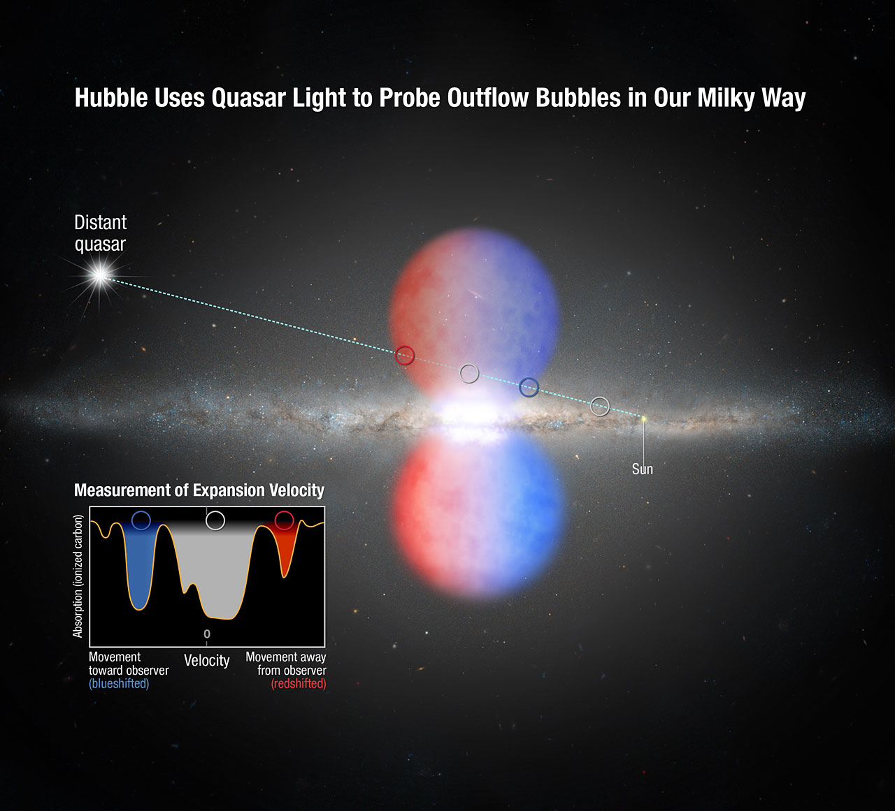
What to notice: background quasars can act like flashlights shining through the Milky Way’s halo. Absorption lines in their spectra reveal otherwise invisible gas flowing above and below the Galactic disk. (Credit: Course-provided figure)
To map a dusty galaxy, change your wavelength: 21-cm HI traces the gas, infrared traces the stars, and Gaia parallaxes build precise 3-D maps where dust allows.
You want to study the stars packed around the Galactic Center, but visible-light images are mostly dark because dust blocks the view. Which wavelength regime should you choose — visible, infrared, or 21-cm radio — and what would that choice let you measure?
Use infrared if your goal is to see the stars. Infrared light passes through dust much more effectively than visible light, so it reveals the dense stellar cluster near the Galactic Center. Use 21-cm radio if your goal is to map neutral hydrogen gas and measure its Doppler shifts. The key move is matching the wavelength to the observable you need.
The Rotation Curve: Where Dark Matter Shows Up
This is the central argument of the lecture.
The Keplerian Prediction
Pretend for a moment that the Milky Way were like the solar system. In the solar system, the Sun holds all the mass, and the planets orbit in Kepler’s third law:
\[ v_{\text{circ}}(r) = \sqrt{\frac{G M_{\text{enclosed}}}{r}}. \]
If almost all the mass is concentrated at the center (as in the solar system), then the enclosed mass \(M_{\text{enclosed}}\) is effectively constant as you go farther out, and the circular velocity falls as \(v \propto r^{-1/2}\).

What to notice: in a central-mass system like the Solar System, orbital speed decreases with distance. This is the prediction that fails for spiral galaxies with flat rotation curves. (Credit: Illustration: A. Rosen (SVG))
The solar system’s rotation curve is exactly this: Mercury is fast, Neptune is slow, and the pattern is Keplerian.
For the Milky Way, the naive expectation is similar: out past the visible stars and gas, there is no more luminous mass to add, so the enclosed mass should stop growing and the circular velocity should start falling like \(r^{-1/2}\).
The Observation
That prediction fails — not subtly, but dramatically.
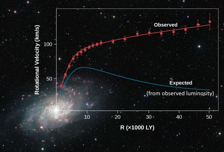
What to notice: the observed rotation curve stays high at large radius, while the curve expected from the observed luminosity alone falls. The gap between those two curves is the dark-matter inference in one picture. (Credit: Course-provided figure)
When we measure the velocity of stars and 21-cm HI gas as a function of radius in the Milky Way (and in every other spiral galaxy we have checked carefully), we find the rotation velocity stays roughly flat out to the edge of detectable gas. Typical disk rotation speeds are ~200 – 250 km/s, and they do not drop off in the way a mass-at-the-center model predicts.
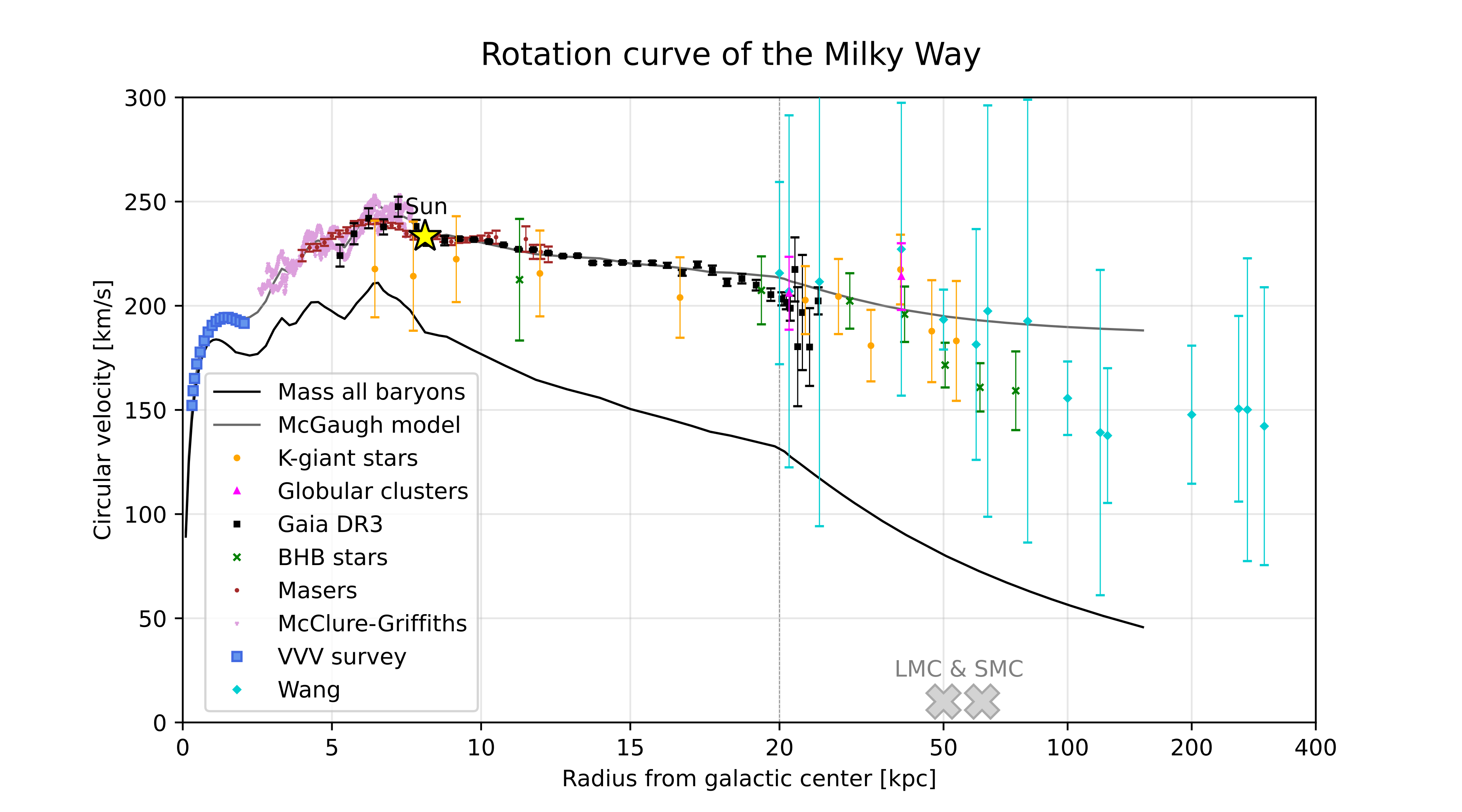
What to notice: many independent tracers of the Milky Way’s rotation stay near the same circular speed even far from the Galactic Center. The baryonic-mass curve falls, so the measured speeds require additional mass. (Credit: Course-provided figure)
The Milky Way version matters because it is not one instrument, one star, or one modeling choice. The same story appears when astronomers use many tracers — stars, masers, globular clusters, Gaia motions, and gas — to measure circular speed at different radii. The scatter and error bars are real; the central pattern is still clear.
The Inference
A flat rotation curve means \(M_{\text{enclosed}}(r)\) keeps growing with radius — linearly, in fact — out past where we can see stars. There is mass out there. It does not emit light. It does not absorb light. It does not scatter light. But it has gravity.
This is the minimal inference from rotation curves. We call the extra mass dark matter, but that name is a placeholder for the observation, not a description of the physics.
The dark matter halo is inferred to be roughly spherical, to extend well beyond the visible disk, and to contain several times more mass than all the stars, gas, and dust combined. In the Milky Way specifically, current estimates place the total mass (dark matter included) at ~10¹² M☉, of which only ~5 – 10% is baryonic.
Observable: The rotation velocity of stars and 21-cm HI gas is approximately constant as a function of radius, out to the edge of detectable gas.
Model: Newtonian gravity applied to a rotating system: \(v_{\text{circ}}^2 = G M_{\text{enclosed}}(r) / r\). A constant \(v_{\text{circ}}\) requires \(M_{\text{enclosed}} \propto r\) — more mass than the stars, gas, and dust contain.
Inference: Either the Milky Way contains a large halo of non-luminous matter (“dark matter”), or the law of gravity we are applying is wrong on galactic scales. The weight of evidence — including, as we will see in Lectures 24 – 26, evidence at much larger scales — favors dark matter.
What would change our mind? A direct particle detection would not be required to justify the gravitational inference, but it would identify the substance. A modified-gravity theory would have to do more than fit one rotation curve: it would need to explain galaxy rotation curves, galaxy clusters, gravitational lensing, the CMB, and the growth of the cosmic web with one coherent model. That is why dark matter is not a single-observation guess; it is the simplest explanation that survives many independent tests.
Suppose two galaxies both have flat rotation curves, but Galaxy A stays flat at 150 km/s while Galaxy B stays flat at 300 km/s. At the same radius, which galaxy has more enclosed mass? By what factor?
Galaxy B has more enclosed mass. From \(M_{\text{enc}} = v^2 r/G\), mass scales as \(v^2\) at fixed radius. Doubling the circular speed from 150 km/s to 300 km/s means \(2^2 = 4\) times more enclosed mass. The observable is velocity; the inference is gravitational mass.
WRONG. “Dark” here does not mean “black” or “dusty.” It means “does not interact with light in any detectable way.” Dust absorbs and scatters visible photons enthusiastically — that’s why the Galactic Center is hidden from us in the optical. Dark matter does neither, which is precisely why it’s so hard to find. We know dark matter exists from its gravity alone.
WRONG in the main. Stellar-mass black holes, rogue planets, neutron stars, and faint stars are all made of the same ordinary atoms that make up you, me, and the Sun — they are baryonic matter. Dedicated searches (microlensing surveys like OGLE and MACHO) have placed tight limits on how much of the halo can be locked up in such compact baryonic objects: nowhere near enough to explain rotation curves. The dark matter problem is not solved by adding up the invisible baryons we haven’t found yet.
What Dark Matter Might Be
Honest answer: we do not know. The leading candidates are:
- Weakly Interacting Massive Particles (WIMPs): hypothetical elementary particles that interact through gravity and the weak force but not electromagnetism. Decades of direct-detection experiments (XENON, LUX, PandaX) have placed extremely tight limits without a confirmed detection.
- Axions: hypothetical very-low-mass particles predicted by certain solutions to problems in particle physics. Experiments like ADMX search for them.
- Primordial black holes: black holes formed in the very early universe (not by stellar collapse). Some mass windows are ruled out; others remain open.
- Modified Newtonian Dynamics (MOND) and related theories: alternatives to dark matter that modify the law of gravity at low accelerations. MOND fits individual galaxy rotation curves very well but struggles with galaxy clusters, the CMB, and the overall cosmological record.
The identity of dark matter is one of the great unsolved problems of physics, and you will hear about it again in Lectures 24 – 26 when we meet it at larger scales.
Flat rotation curves demand more mass than we can see. That extra mass, whatever it is, is what we call dark matter.
Sagittarius A*: Weighing the Monster at the Center
If you look toward the constellation Sagittarius with a radio telescope, you find a bright, compact radio source called Sagittarius A* (pronounced “Sag A-star”). It is small, it does not move, and for decades it was one of the most mysterious points in the sky.
What lives there? The answer came from stellar orbits.
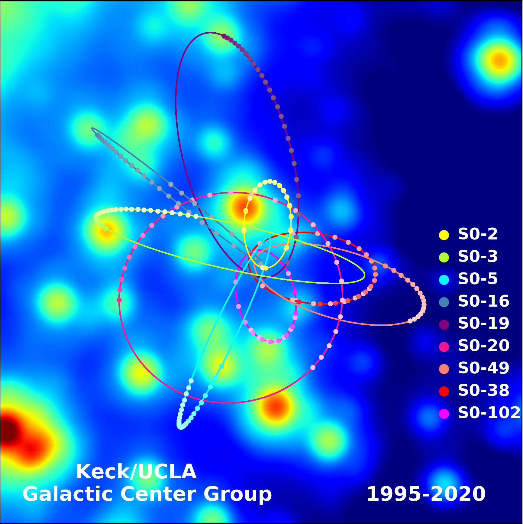
What to notice: the stars do not drift randomly. They trace closed, high-speed orbits around a common focus, which lets astronomers weigh the compact object at the Galactic Center with Kepler’s third law. (Credit: Keck/UCLA Galactic Center Group)
Use the slider to watch the Galactic Center observations build up from 1998 to 2009. Before you move the slider, predict what kind of pattern would convince you that the stars are orbiting one compact central mass rather than drifting randomly.
What to notice: the observable is not the black hole itself. It is the changing positions of nearby stars. The model is orbital motion under gravity. The inference is that millions of solar masses must be packed inside the shared focus of those orbits.
The S-Stars
Over two decades, groups led by Andrea Ghez (UCLA) and Reinhard Genzel (MPI) tracked a small cluster of stars — the S-stars — orbiting something at the Galactic Center. One of them, S2 (also called S0-2), has an orbital period of about 16 years and a closest approach of ~120 AU. It was observed across a full orbit. Ghez and Genzel shared the 2020 Nobel Prize in Physics for this work.
If you have an orbiting star, you can apply Kepler’s third law (callback to Lecture 5) to infer the mass it is orbiting.
Worked Example: The Mass of Sgr A*
Given: Star S2 orbits Sgr A* with period \(P \approx 16\) yr and semi-major axis \(a \approx 970\) AU (about 1,000 AU, to one significant figure).
Relation: Kepler’s third law, in units where \(P\) is in years, \(a\) is in AU, and \(M\) is in \(M_\odot\):
\[ \frac{M_{\text{Sgr A*}}}{M_\odot} = \frac{(a/\text{AU})^3}{(P/\text{yr})^2} \]
(This is Kepler’s third law in solar-system units, with the companion-star mass negligible.)
Substitute:
\[ \frac{M_{\text{Sgr A*}}}{M_\odot} = \frac{(970)^3}{(16)^2} \]
Evaluate:
\[ \frac{M_{\text{Sgr A*}}}{M_\odot} \approx \frac{9.1 \times 10^8}{256} \approx 3.6 \times 10^6 \]
Interpretation: Sgr A* has a mass of roughly \(4 \times 10^6\ M_\odot\) (the current best value is \(4.3 \times 10^6\ M_\odot\)). The mass is concentrated inside a region small enough that S2 can swing within ~120 AU without running into it.
What else could this be? A four-million-solar-mass cluster of ordinary stars inside that volume would be so dense that internal collisions would disperse it on timescales much shorter than the age of the galaxy. A cluster of neutron stars or stellar-mass black holes of that total mass runs into the same problems. The only thing we know that can pack \(4 \times 10^6\ M_\odot\) into a volume smaller than our solar system is a supermassive black hole.
Supermassive black hole (SMBH): A black hole with mass of \(10^5\) to \(10^{10}\ M_\odot\). Most massive galaxies examined carefully appear to host one near their center.
In May 2022, the Event Horizon Telescope released the first direct image of Sgr A*’s shadow. The angular size of that shadow matches, to within measurement uncertainty, the size predicted by the orbit-derived mass and the Schwarzschild-radius formula from Lecture 21.
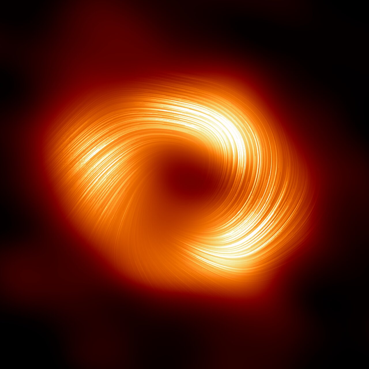
What to notice: this is a horizon-scale radio image of Sgr A* in polarized light. The bright ring surrounds the black-hole shadow, and the fine lines trace polarization directions related to magnetic fields near the event horizon. (Credit: EHT Collaboration)
The polarized-light view shown here is a later EHT result, so keep the chronology straight: the mass of Sgr A* came first from stellar orbits, the 2022 image checked the predicted shadow scale, and the polarized image adds information about magnetic fields near the event horizon.
Polarization is also a nice example of the course throughline at work. We do not see magnetic fields directly. We infer their geometry from how light is polarized by plasma near the black hole and by dust grains across the Milky Way.
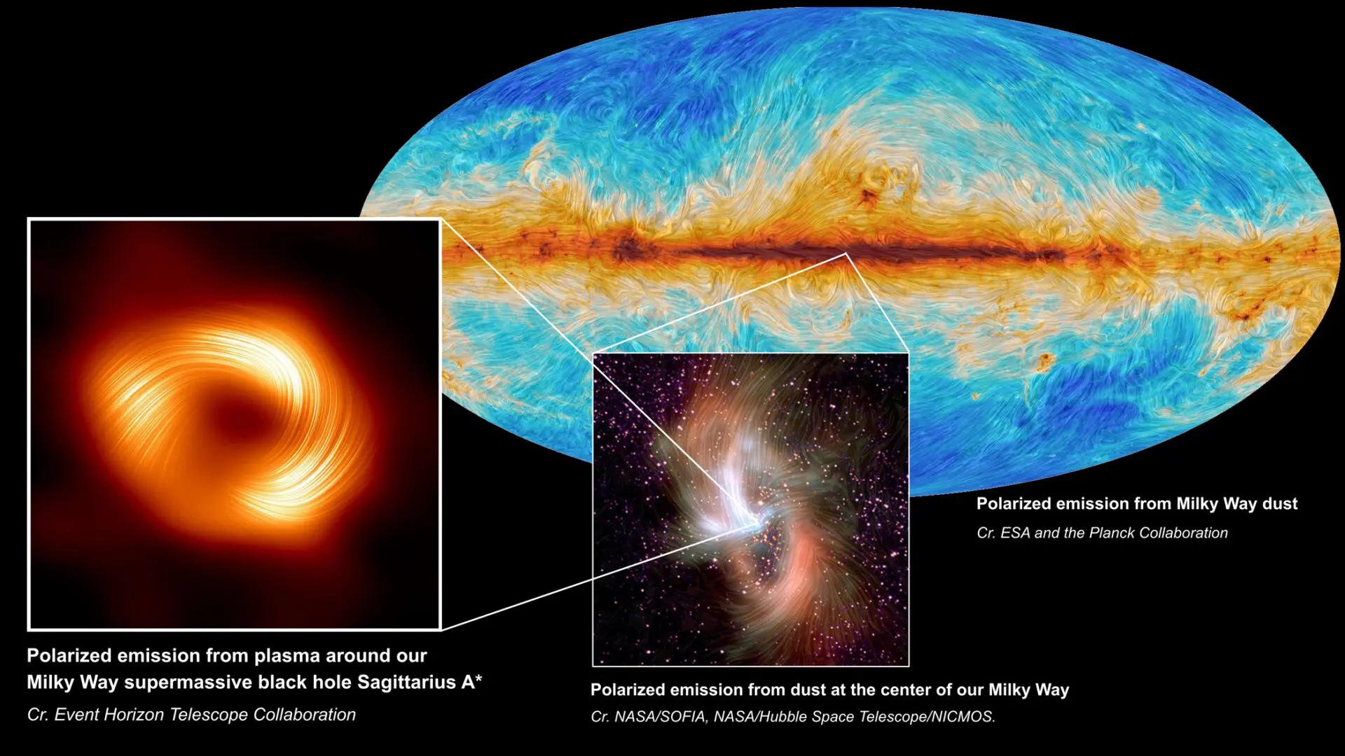
What to notice: polarization is a magnetic-field tracer across enormous scale ranges. The same technique links plasma near Sgr A*, dust near the Galactic Center, and polarized dust emission across the Milky Way. (Credit: Event Horizon Telescope Collaboration; NASA/SOFIA; NASA/Hubble Space Telescope/NICMOS; ESA and the Planck Collaboration)
Using the Schwarzschild-radius formula from Lecture 21, \(R_S = 2GM/c^2\), estimate the Schwarzschild radius of Sgr A* in AU. For \(M = 4 \times 10^6 \, M_\odot\), \(R_S\) in meters is about \(2 \times (6.67 \times 10^{-11}) \times (4 \times 10^6 \times 2 \times 10^{30}) / (3 \times 10^8)^2\). Convert the final answer to AU using \(1\,\text{AU} \approx 1.5 \times 10^{11}\) m.
Given: \(M = 4 \times 10^6 M_\odot = 8 \times 10^{36}\) kg.
Evaluate the formula:
\[ R_S = \frac{2 \times (6.67 \times 10^{-11}) \times (8 \times 10^{36})}{(3 \times 10^8)^2} \approx \frac{1.07 \times 10^{27}}{9 \times 10^{16}} \approx 1.2 \times 10^{10} \text{ m}. \]
Convert: \(R_S \approx 1.2 \times 10^{10} \, \text{m} / (1.5 \times 10^{11} \, \text{m/AU}) \approx 0.08\) AU.
Interpretation: The event horizon of Sgr A* is roughly 0.08 AU in radius — about one-tenth of the Earth-Sun distance. The S-stars orbit well outside this, but close enough that their motion is unmistakable gravitational evidence for a SMBH.
The orbits of a few stars, combined with Kepler’s third law, weigh Sgr A* at \(\sim 4 \times 10^6\ M_\odot\) and pack that mass into a region small enough to be nothing but a supermassive black hole.
The Distance-Ladder Check-In
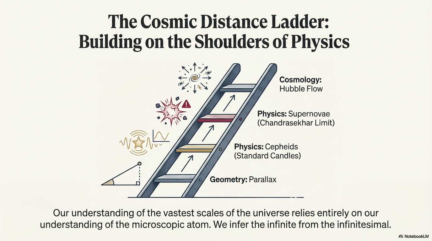
What to notice: Each rung calibrates the next. Parallax (geometry) → Cepheids (standard candles) → Supernovae (Chandrasekhar limit) → Hubble Flow (cosmology). We infer the infinite from the infinitesimal. (Credit: (A. Rosen/NotebookLM))
Here is where we stand on the cosmic distance ladder at the end of this lecture:
- Rung 1 (radar, AU): solar system, established Module 1.
- Rung 2 (parallax, pc to kpc): nearby stars and much of the Gaia sample, established Lecture 15.
- Rung 3 (main-sequence fitting / spectroscopic parallax, kpc): globular clusters and distant open clusters within the Milky Way, established Lecture 16.
Everything we said today about the Milky Way relies on these three rungs. We have not yet built a rung that reaches other galaxies. That is the work of Lectures 23 and 24.
Our map of the Milky Way is built from the bottom three rungs of the distance ladder — and all three rely on stars.
Deep Dive: How Do You Actually Measure a Rotation Curve?
To turn a galaxy image into a rotation curve you need two things: distances along the line of sight, and velocities along the line of sight. Neither is trivial when you live inside the object you are trying to measure.
For our galaxy specifically, the approach for the outer disk is as follows. 21-cm HI emission lets us detect neutral hydrogen at high resolution anywhere in the disk, including through the dust. Doppler shifts of the 21-cm line give us the HI’s line-of-sight velocity. For clouds that we can geometrically constrain to be on circular orbits, the line-of-sight velocity and the cloud’s Galactic longitude combine (through a kinematic model) to give its circular speed. Repeating this across many longitudes yields the rotation curve.
For other spiral galaxies — the ones we see face-on or moderately inclined — the approach is similar: 21-cm HI emission, sometimes supplemented by optical emission lines from H II regions, gives velocity fields that are deprojected to recover the underlying circular velocity as a function of radius.
You do not need to know the detailed kinematic modeling to grasp the inference. The point is that rotation curves are real measurements, built from real stars and real gas, using the same Doppler and spectral-line physics you met in Module 1.
Deep Dive: Other Lines of Evidence for Dark Matter
Rotation curves are the classic evidence students meet first. They are not the only evidence. Other lines include:
- Galaxy cluster velocity dispersions (Zwicky, 1933): galaxies in the Coma cluster move faster than the cluster’s visible mass can account for; most of the cluster mass must be dark. This is actually the original dark-matter argument, predating galaxy rotation curves by decades.
- Gravitational lensing: mass bends light. Maps of the total mass in clusters, inferred from lensing of background galaxies, disagree dramatically with maps of the visible mass. The famous “Bullet Cluster” image shows the separation between the two.
- Structure formation in cosmological simulations: the pattern of galaxy clustering we see today requires a dominant cold, non-baryonic matter component to form on the right timescale. Baryons alone cannot do it.
- The cosmic microwave background: (Lecture 26) the CMB’s acoustic-peak structure independently constrains the ratio of dark matter to baryons and agrees with the galactic evidence.
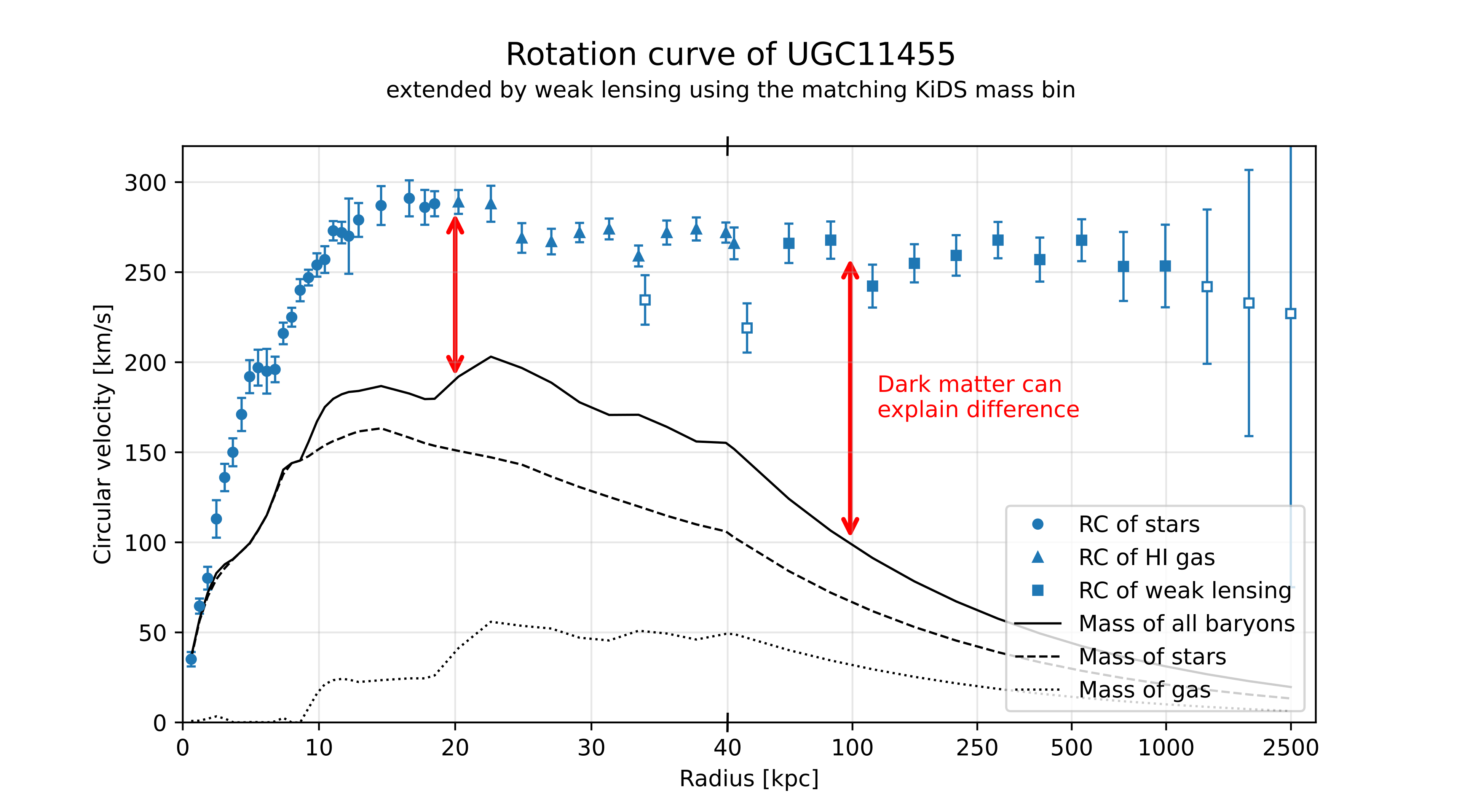
What to notice: UGC 11455 rotates faster than its baryonic mass can explain, and weak lensing extends the same mass discrepancy to much larger radii. Dark matter is not just a Milky Way bookkeeping problem. (Credit: Course-provided figure)
This figure previews how the argument scales up. The inner points are rotation-curve measurements, like the ones we just discussed. The far-out weak-lensing points ask a different question: how much total mass bends background light around the galaxy? The two methods do not measure the same thing in the same way, but they point toward the same conclusion: baryonic matter alone is not enough.
The Bullet Cluster is the same kind of evidence, but with an even cleaner separation. In a galaxy-cluster collision, most of the ordinary matter is hot gas. The gas collides, slows down, and glows in X-rays. The galaxies and dark matter mostly pass through. Gravitational lensing then shows where the mass went.
What to notice: the pink X-ray gas marks much of the ordinary matter, while the blue lensing map marks where most of the gravitating mass is. Their separation is why the Bullet Cluster is a clean dark-matter test. (Credit: NASA/CXC/CfA/STScI/ESO/Magellan)
The newer multi-observatory view below makes the same point with a richer field. Do not try to memorize the colors; ask what each layer is tracing. Galaxies mark where stars are, X-rays mark hot gas, and lensing marks total gravitating mass.
What to notice: multi-observatory images separate luminous galaxies, hot gas, and lensing mass. The dark-matter argument is strongest because different messengers point to different physical components. (Credit: Course-provided figure)
Use the wavelength controls to compare the visible galaxies, the X-ray-emitting gas, and the lensing-based mass map. This is the cleanest place in the module to see why dark matter is not just “stuff we forgot to count.”
What to notice: the hot ordinary gas slows down during the cluster collision, while the lensing mass map is displaced from that gas. The separation between normal matter and gravitational mass is why the Bullet Cluster is such an important independent line of evidence.
No single observation proves dark matter. The case is built from many independent observations at very different scales pointing to the same conclusion.
Misconceptions
WRONG. Until the 1920s, many astronomers believed the Milky Way was the universe, and that “spiral nebulae” were just nearby objects. Edwin Hubble’s 1924 measurement of the distance to the Andromeda Nebula (M31) showed it was hundreds of times farther than the edge of the Milky Way — that is, it was another galaxy. We are one of hundreds of billions.
WRONG. We cannot see the Milky Way from the outside, but we can build its map using 21-cm HI kinematics, infrared star counts, Gaia parallaxes and proper motions, and stellar spectroscopy. The map is incomplete and will improve with Rubin and next-generation radio surveys, but it is not blind.
WRONG (but common in 1915). The Sun is ~8 kpc from the center, in the disk, roughly halfway out. The interstellar dust hid this fact from early optical astronomers. Harlow Shapley established the Sun’s off-center position in the 1910s using globular-cluster distances — a beautiful early example of using stellar populations to map galactic structure.
Practice Problems
Solutions are available in the Lecture 22 Solutions.
Core Problems (Start Here)
Problem 1: Identifying Populations. For each Milky Way component (disk, bulge, halo, spiral arms), name whether you expect to find more young O/B stars or more old K/M stars, and explain your reasoning in one sentence.
Problem 2: Wavelength Choice. You want to map gas in the Galactic disk behind the dense dust of the Galactic Center. Which is better — visible light, 21-cm radio, or near-infrared? Justify your answer.
Problem 3: Reading a Rotation Curve. You observe a spiral galaxy whose rotation curve rises from the center out to 3 kpc, then stays flat at 220 km/s out to at least 15 kpc. Sketch the visible-mass prediction and the observed curve on the same axes, and mark where “extra mass” is required.
Problem 4: Enclosed Mass from a Rotation Curve. The Milky Way’s rotation curve is roughly flat at \(v \approx 220\ {\rm km\,s^{-1}}\). At a radius \(r = 20\ {\rm kpc}\), estimate the enclosed mass in solar masses using \(M_{\text{enc}} = v^2 r / G\). Useful conversion: \(G \approx 4.3 \times 10^{-6}\ {\rm kpc}\,({\rm km\,s^{-1}})^2\,M_\odot^{-1}\).
Problem 5: Weighing Sgr A*. Star S2 is observed to orbit the Galactic Center with period \(P \approx 16\ {\rm yr}\) and semi-major axis \(a \approx 970\ {\rm AU}\). Using Kepler’s third law in solar units, estimate the central mass. Your answer should be close to the mass of Sgr A* from the worked example.
Challenge Problems (Deepen Your Understanding)
Challenge 1: Schwarzschild Radius Scaling. Show that for a black hole of mass \(M\), the Schwarzschild radius \(R_S = 2GM/c^2\) scales linearly with mass. If a \(10\ M_\odot\) stellar-mass black hole has \(R_S \approx 30\ {\rm km}\), what is \(R_S\) for Sgr A* (\(4 \times 10^6\ M_\odot\))? Compare to your answer from Check Yourself 4.
Challenge 2: Dark Matter vs. MOND. Write a one-paragraph argument explaining why a single well-measured rotation curve is not, by itself, enough to distinguish dark matter from MOND. What additional observations would help?
Challenge 3: What Fraction Is Baryonic? Suppose all the stars in the Milky Way total \(\sim 6 \times 10^{10}\ M_\odot\), and all the gas totals another \(\sim 10^{10}\ M_\odot\). If the total mass enclosed within \(100\ {\rm kpc}\) is \(\sim 10^{12}\ M_\odot\) (dominated by dark matter), what fraction of the Milky Way’s mass is luminous?
Reading Summary
- The Milky Way is a barred spiral with a disk, bulge/bar, halo, and spiral arms; each component hosts a characteristic stellar population that records a different chapter of galactic history.
- We map our dusty galaxy by changing wavelength: 21-cm HI emission traces the gas, infrared traces the stars behind the dust, and Gaia parallaxes build precise 3-D maps in the optical.
- Spiral galaxies, including the Milky Way, have flat rotation curves — \(v_{\text{circ}}(r)\) does not fall off like \(r^{-1/2}\) past the visible edge. Newtonian gravity then requires \(M_{\text{enclosed}}(r) \propto r\), i.e., non-luminous mass far outside the stars. That mass is called dark matter.
- Stellar orbits near the Galactic Center obey Kepler’s third law and give \(M_{\text{Sgr A*}} \approx 4 \times 10^6\,M_\odot\) in a volume smaller than the solar system — an unambiguous supermassive black hole.
- Distance-ladder status: radar → parallax → main-sequence fitting. Everything we said about the Milky Way depends on these three rungs. Lectures 23 – 24 extend the ladder beyond our galaxy.
Glossary
21-cm line: Radio emission from neutral hydrogen produced by the hyperfine spin transition. It lets astronomers map HI gas through dust.
Bulge/bar: The dense central stellar region of the Milky Way. In our galaxy, the inner bulge is elongated into a rotating bar.
Dark matter: Matter inferred from gravity that does not emit, absorb, or scatter light detectably. In this lecture, the key evidence is the Milky Way’s flat rotation curve.
Disk: The flattened, rotating component of the Milky Way containing most of its gas, dust, young stars, and spiral arms.
HI: Neutral atomic hydrogen. The notation means hydrogen whose electron is still bound to the proton, rather than ionized.
Infrared: Light with wavelengths longer than visible red light. Infrared observations can reveal stars and warm dust in regions where visible light is blocked.
Interstellar dust: Tiny solid grains mixed with gas between stars. Dust absorbs and scatters visible light, especially toward the Galactic Center.
Milky Way: Our home galaxy, a barred spiral galaxy containing the Sun, stars, gas, dust, dark matter, and Sagittarius A* at its center.
Modified Newtonian Dynamics (MOND): A class of alternatives to dark matter that modifies gravity or inertia at very low accelerations.
Rotation curve: A plot of orbital speed versus distance from a galaxy’s center. A flat rotation curve means orbital speed stays roughly constant at large radius.
Sagittarius A*: The compact radio source at the center of the Milky Way associated with the galaxy’s central supermassive black hole.
Schwarzschild radius: The event-horizon radius of a non-rotating black hole, given by \(R_S = 2GM/c^2\).
Spiral arm: A density-wave pattern in a galactic disk, traced by gas, dust, young massive stars, and H II regions.
S-stars: Stars on tight orbits around Sagittarius A*. Their motions provide the strongest stellar-orbit evidence for the Milky Way’s central black hole.
Stellar halo: The sparse, roughly spherical population of old stars, globular clusters, and dwarf-galaxy debris surrounding the Milky Way’s disk.
Looking Ahead
Next lecture (Lecture 23), we zoom out to the galaxy zoo — how we classify galaxies, how they differ, and what the extraordinarily luminous quasars at their centers are. We will meet the other supermassive black holes: not ours, but the more massive and more active ones in other galaxies, and we will preview the distance-ladder problem that Lecture 24 will solve.
After that, the distance ladder gets its proper treatment (Lecture 24), Type Ia supernovae reveal the accelerating universe (Lecture 25), and the cosmic microwave background and Big Bang nucleosynthesis reveal our origins (Lecture 26).
Dark matter is the first of three hidden things. We will meet dark energy in Lecture 25 and the origin of the elements in Lecture 26. By the end of this module, the Milky Way will no longer feel like a lonely island — it will feel like a chapter in a much larger story.