Lecture 17: Binary Stars & Stellar Masses
Mass Is Destiny
The Big Idea
You cannot directly weigh a star — unless it has a dance partner. A large fraction of stars, especially higher-mass stars, live in binary or multiple systems, and by watching them orbit under gravity we can unlock the single most important property in stellar astronomy: mass. Mass is destiny in the universe of stars.
This reading answers three questions:
- How do visual, eclipsing, and spectroscopic binaries let us measure stellar masses?
- What do those masses teach us about the mass-luminosity relation?
- Why does mass control stellar lifetime and stellar fate?
Default expectation (best): Read the whole page before lecture and stop at the check-yourself prompts.
If you’re short on time (~20 min):
- Focus on the three binary types, Newton’s version of Kepler’s Third Law, and the mass-luminosity relation.
- Return to the challenge problems after class.
Reference mode: Use the summary, glossary, and solutions companion when later readings start using stellar mass as the organizing variable.
Opening: The Dance Partners Problem
Suppose I show you a star 100 light-years away. Name one property you could measure from its light, and explain why mass would still be hidden.
Imagine trying to weigh a distant star. You cannot put it on a scale. You cannot bring it to a laboratory. Yet astronomers know the masses of many stars — often to within a few percent accuracy in the best binary systems. How?
The answer lies in gravity and geometry. Whenever two stars orbit each other, they create a natural laboratory for measuring mass. Their dance around a shared center reveals the gravitational pull between them, which depends on how much mass each star contains. By careful observation of this dance, we can work backward to find the masses of both stars.
Astronomy often works by turning invisible quantities into measurable motion. In binary systems, gravity turns stellar mass into orbital behavior.
This is one of the most powerful techniques in astronomy because it turns motion into physics. A large fraction of stars are not alone, and those partnered stars let gravity do the weighing for us.
Binary star system: Two stars orbiting a shared center of mass under mutual gravity. Three or more stars form a “multiple system.”
Why Mass Matters: The Central Message
Before we learn how to measure mass, we need to understand why it matters so much.
In previous lectures, we learned that stars fuse hydrogen into helium in their cores. We learned that the Sun has fused quietly for about 5 billion years and will continue for another 5 billion more. But not all stars live at the Sun’s pace. Some burn out in just a few million years. Others glow steadily for hundreds of billions of years — far longer than the current age of the universe. The difference? Mass.
Mass is the primary variable in stellar physics. It determines:
- How luminous a star is: More massive stars are vastly brighter.
- How hot a star burns: More massive stars have hotter cores and burn hydrogen faster.
- How long a star lives: More massive stars use up their fuel much more quickly — they “live fast and die young.”
- What the star becomes when it dies: A 10-solar-mass star explodes as a supernova; the Sun will fade as a white dwarf.
The rough relationship is elegant: a star’s mass sets its luminosity, which sets how fast it burns fuel, which sets how long it survives. Understanding mass is the master key to understanding stars.
You can summarize the chain in one line:
birth mass -> core pressure and temperature -> fusion rate -> luminosity -> lifetime -> final fate
Mass is destiny. A star born with 10 times the Sun’s mass will be roughly 3000 times more luminous and live only about 30 million years instead of about 10 billion. Everything flows from mass.
But here is the problem: we cannot measure mass directly. We can measure a star’s brightness, its color, its spectrum, even its radius in a few special cases. In general, stellar mass cannot be measured directly from brightness or spectrum alone; for most single stars it must be inferred indirectly using relations calibrated by binary systems.
This is where binary stars become indispensable.
If stellar mass increases by a lot, which should change more dramatically: the available fuel supply or the luminosity? Explain your reasoning in one sentence.
Mass is the control knob of stellar physics: it sets a star’s luminosity, lifetime, and end state.
Binary Stars: Nature’s Mass Measuring Tool
A large fraction of stars — especially higher-mass stars — exist in binary or multiple systems rather than as solitary stars. Some binaries are easy to see as two separated points of light. Others are detected only through subtle Doppler shifts in their light or periodic dimming caused by one star passing in front of the other. Regardless of how we detect them, binary systems all share one crucial property: they let us connect motion to mass.
The logic is simple. Two stars orbit each other under mutual gravity. Their orbital period and separation tell us the total mass they contain. If the two stars orbit differently — one moving faster than the other, or one traveling on a wider orbit than the other — we can infer how that total mass is divided between them.
Let’s examine the three main types of binaries and what we learn from each.
If two stars orbit the same center of mass in the same period, which one must move faster: the more massive star or the less massive star? Explain why.
Use the interactive below to connect the reading’s main idea to actual orbital motion. As you change the masses and viewing geometry, notice which star moves faster, which orbit is larger, and how the center of mass stays fixed.
Try these quick checks:
- Make one star much more massive than the other. Which orbit gets smaller, and which star moves faster?
- Set the two stars to equal mass. What changes about the two orbits?
- Change the viewing angle or turn on any radial-velocity options. Which observables would help you most: position on the sky, brightness dips, or Doppler motion?
Visual Binaries: Seeing Both Stars Orbit

What to notice: equal masses place the center of mass halfway; unequal masses move it toward the larger body. (Credit: cococubed.com)
A visual binary is a system where both stars are bright enough and far enough apart that ground-based or space telescopes can resolve them as separate objects. Astronomers have been tracking some visual binaries for centuries, building up precise measurements of their projected orbits on the sky.
The most famous example is Sirius, the brightest star in Earth’s night sky. In the early 1800s, Friedrich Wilhelm Bessel noticed that Sirius seemed to wiggle back and forth slightly as it moved across the sky. He realized the bright star was being gravitationally tugged by an invisible companion. In 1862, a telescope finally revealed the companion: Sirius B, a faint, tiny star.
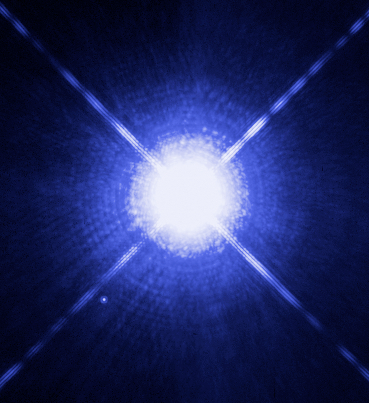
What to notice: Sirius B is easy to miss next to the glare of Sirius A, but resolving the pair visually is what turns a point of light into a measurable gravitational system. (Credit: NASA/ESA/Hubble)
To find the masses of Sirius A and B, astronomers observed their positions over decades. Both stars trace elliptical paths projected on the sky. For visual binaries, the orbit is measured in angular units on the sky, so astronomers must know the distance in order to convert that angular size into a physical size in AU.
Once that conversion is in hand, we use Newton’s solar-unit form of Kepler’s third law:
\[ M_1 + M_2 = \frac{a^3}{P^2} \]
- \(a\) = semi-major axis of the relative orbit in AU
- \(P\) = orbital period in years
- \(M_1 + M_2\) = total mass in solar masses (\(M_\odot\))
In this solar-unit form, \(a\) refers to the semi-major axis of the relative orbit; for a circular orbit, this is the average separation between the stars.
This equation returns the total mass of the binary system. By itself, it does not yet tell us how that total is split between the two stars.
In the solar-unit form of Kepler’s third law, \(a\) must be in \(\mathrm{AU}\), \(P\) must be in \(\mathrm{yr}\), and the resulting mass is in \(M_\odot\). If you feed in arcseconds or days without converting, the answer will be wrong.
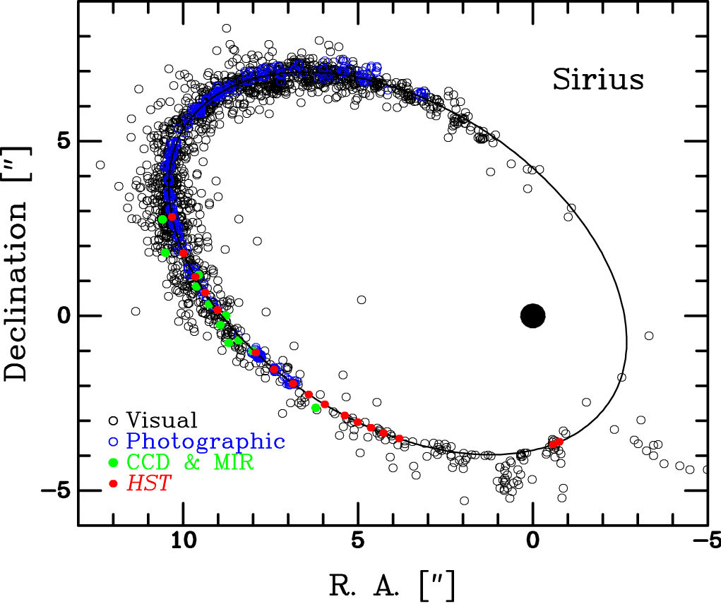
What to notice: measuring stellar masses is often slow astronomy. Decades of astrometric points trace Sirius B’s orbit around Sirius A and reveal the period, separation, and center-of-mass geometry needed for the mass calculation.
Visual binaries can give the total mass from orbit size plus period, but only after angular measurements on the sky are converted into a physical orbit in AU using the system’s distance.
For Sirius, the orbital separation is roughly \(a = 20 \, \mathrm{AU}\) and the period is \(P = 50 \, \mathrm{yr}\). We can write the calculation in full physics grammar:
General relation
\[ M_1 + M_2 = \frac{a^3}{P^2} \]
- \(a\) = \(20 \, \mathrm{AU}\)
- \(P\) = \(50 \, \mathrm{yr}\)
- \(M_1 + M_2\) = total system mass in \(M_\odot\)
Substitute the measured values
\[ M_1 + M_2 = \frac{(20 \, \mathrm{AU})^3}{(50 \, \mathrm{yr})^2} \]
Evaluate
\[ M_1 + M_2 = \frac{(20 \, \mathrm{AU})^3}{(50 \, \mathrm{yr})^2} = 3.2 \, M_\odot \]
The Sirius binary contains about \(3.2 \, M_\odot\) total.
Does this answer make physical sense? Yes. Sirius A is an A-type main-sequence star and Sirius B is a white dwarf companion, so a few solar masses total is a reasonable scale for the system.
To go from total mass to individual masses, astronomers need one more geometric clue: how far each star orbits from the center of mass. The more massive star orbits closer to that center; the less massive star orbits farther away. Measuring those orbit sizes gives the mass ratio, and combining that ratio with the total mass gives the individual masses.
If one star traces the larger orbit around the center of mass, what does that tell you about its mass? Explain, not just which star it is.
Center of mass: The point that both stars orbit. It lies closer to the more massive star. The balance condition is \(M_1 d_1 = M_2 d_2\), where \(d_1\) and \(d_2\) are distances from the center of mass.
“If I can see both stars, I automatically know both masses.” Not quite. Seeing the orbit gives the total mass only after the angular orbit is converted to AU, and individual masses require the center-of-mass geometry as well.
Visual binaries give total mass from orbital size and period once distance is known well enough to convert the orbit into AU; with center-of-mass information, they can also give the mass ratio.
Eclipsing Binaries: Stars in Shadow
Some binary systems are oriented so that their orbital plane points nearly edge-on toward us. When this happens, one star periodically passes directly in front of the other. We see the combined brightness dip when the dimmer star is hidden behind the brighter one — and again when the brighter star eclipses the dimmer one.
These eclipsing binaries are especially valuable because the eclipse geometry tells us the orbit is nearly edge-on. That sharply constrains the inclination, which is exactly the geometric information that spectroscopic binaries often lack.
If one star is much hotter and brighter than its companion, during which eclipse should the total light drop more? Explain what the light curve is telling you.
Here is why. As one star passes in front of the other, it takes a certain amount of time for the eclipse to complete. The timing of ingress, totality, and egress depends on the orbital speed and on the sizes of the stellar disks. The depth of each dip depends on how much light is being blocked.
The deeper eclipse happens when the hotter, brighter star is hidden, because that is when the system loses the larger share of its total light.
The most famous eclipsing binary is Algol (Beta Persei), known since ancient times as the “Demon Star” because its brightness visibly pulses. Its brightness drops to about 1/3 its normal value for about 10 hours every 2.87 days — a pattern that repeats like clockwork.

What to notice: the deeper dip happens when the hotter, brighter star is blocked. The shallower dip happens when the cooler star is hidden. Dip depth and width encode temperature contrast, orbital geometry, and stellar size. (Credit: Gemini Observatory)
From the light curve of Algol — the graph of brightness versus time — astronomers measure:
- The orbital period
- How much the brightness drops during each eclipse
- How long each eclipse lasts
- The relative timing of the two eclipses during one orbit
A light curve by itself usually does not give precise stellar masses. Its power is that it strongly constrains the orbital inclination and the relative sizes and surface-brightnesses of the stars. When those constraints are combined with spectroscopic radial velocities, astronomers can determine accurate masses and radii.
That is why eclipsing systems are so prized: they pin down geometry that other methods leave uncertain.
In Algol, the brighter star (Algol A) is now more massive than its companion, while the fainter star (Algol B) is less massive but more evolved. That is the famous clue that Algol has not evolved like two isolated stars.
This is the Algol paradox. In a single-star picture, the more massive star should evolve first. But in Algol, the less massive star looks more evolved. The resolution is mass transfer: Algol B used to be the more massive star, evolved faster, expanded, and lost mass to Algol A. Today Algol A is more massive, while Algol B looks too evolved for its current mass.
Eclipsing binaries strongly constrain inclination and stellar radii from the light curve, but precise masses usually require spectroscopic radial velocities too.
Spectroscopic Binaries: Reading the Wobbling Light
Many binary stars are too close together for any telescope to resolve them as separate objects. A telescope sees them as a single point of light. Yet they are still detectable — through the Doppler effect applied to their spectra.
As two stars orbit each other, sometimes one is moving toward us while the other moves away from us. A spectroscopic binary reveals itself through periodic shifts in the wavelengths of absorption lines in its spectrum.
The advantage of spectroscopic binaries is that they are numerous. Close binary systems are common, and even when the stars blur into one point of light, the spectrum can still reveal the orbit.
The radial-velocity curve — a graph of velocity versus time — tells us:
- The orbital period
- The radial velocity amplitude of each star
- Which star is moving toward us or away from us at a given time
Radial velocity: The component of a star’s velocity along the line of sight to us. It is measured from Doppler shift.
Here the velocity amplitude means the maximum line-of-sight speed read from the radial-velocity curve.
If one star’s spectral lines swing through a much larger Doppler shift than the other’s, does that star have the larger mass or the smaller mass? Explain how the center of mass forces that result.
Because both stars orbit the same center of mass in the same period, the more massive star must move more slowly. The center-of-mass condition can be written as:
\[ M_1 v_1 = M_2 v_2 \]
- \(M_1\) and \(M_2\) = the two stellar masses, in any common mass unit
- \(v_1\) and \(v_2\) = orbital speeds or velocity amplitudes, in the same velocity units
- This equation expresses the balance around the center of mass
Solving that relation for the mass ratio gives:
\[ \frac{M_2}{M_1} = \frac{v_1}{v_2} \]
- \(\frac{M_2}{M_1}\) = mass ratio, a dimensionless number
- \(\frac{v_1}{v_2}\) = velocity ratio, also dimensionless
- This equation returns the relative masses of the two stars
The mass ratio is the inverse of the velocity ratio because both stars orbit the same center of mass in the same period. The star with the larger velocity amplitude must be the less massive one.
If the primary star has a velocity amplitude of \(50 \, \mathrm{km\,s^{-1}}\) and the secondary has an amplitude of \(150 \, \mathrm{km\,s^{-1}}\), then
\[ \frac{M_2}{M_1} = \frac{50 \, \mathrm{km\,s^{-1}}}{150 \, \mathrm{km\,s^{-1}}} = 0.33 \]
So Star 2 is about one-third the mass of Star 1.
Does this answer make physical sense? Yes. The star moving three times faster comes out three times less massive, which matches the center-of-mass picture.
Spectroscopic binaries also teach an important caution. Radial velocities measure only motion along our line of sight, so spectroscopic data alone usually give minimum masses unless we also know the orbital inclination from eclipses or some other geometry.
Spectroscopic binaries reveal orbital motion and mass ratios through Doppler shifts, but by themselves they usually give minimum masses rather than fully determined individual masses.
In a spectroscopic binary, you measure one star’s radial velocity amplitude to be \(10 \, \mathrm{km\,s^{-1}}\) and the other’s to be \(40 \, \mathrm{km\,s^{-1}}\). Which star is more massive, and what is the mass ratio? Explain your reasoning.
[Solution] The star with the smaller velocity amplitude is more massive, because the more massive star stays closer to the center of mass and moves more slowly.
Using the inverse mass-velocity relation,
$$ = = = 0.25
$$ The velocity units cancel, leaving a dimensionless mass ratio. The star with the \(10 \, \mathrm{km\,s^{-1}}\) amplitude is the more massive star, and the other star has one-quarter of its mass.
Many Systems Are Multiple Types
Real binary systems are often more informative than the labels make them sound. A system can be visual and spectroscopic, or eclipsing and spectroscopic, or in rare cases all three. That is wonderful news, because each observational method constrains a different part of the problem.
How Each Binary Type Helps Us Weigh Stars
| Binary type | Observable | Physical meaning | Why it matters for mass |
|---|---|---|---|
| Visual | Positions on the sky over time | Orbit shape, period, angular size, center-of-mass geometry | Gives total mass once distance converts the orbit into AU; can give the mass ratio if both orbits are mapped |
| Eclipsing | Brightness dips versus time | Inclination, relative radii, surface-brightness contrast | Removes major geometric uncertainty and, with spectroscopy, helps turn minimum masses into accurate masses |
| Spectroscopic | Doppler shifts of spectral lines | Radial velocities and velocity amplitudes | Gives orbital motion and mass ratio even when the stars are unresolved; usually needs inclination information for precise masses |
Why are eclipsing spectroscopic binaries especially valuable for measuring stellar masses?
[Solution] Spectroscopy gives the orbital velocities and usually the mass ratio, but by itself it often gives only minimum masses because the inclination is unknown. Eclipses show that the orbit is nearly edge-on and constrain the radii from the light curve. Together, the two datasets give the geometry and the motion, which is why eclipsing spectroscopic binaries can yield especially accurate masses and radii.
Binary-star astronomy works because each observable maps to a physical constraint: positions give geometry, eclipses give size and inclination, and Doppler shifts give motion.
Extracting Individual Masses: A Worked Example
This is a toy example inspired by Algol, using rounded numbers for teaching. The goal is to see the logic, not to memorize a specific real system.
Math grammar note: Track both the quantity and the units on each line. The units are not decoration; they tell you whether the equation is being used correctly.
Given
- Orbital period: \(P = 2.87 \, \mathrm{days}\)
- Semi-major axis of the relative orbit: \(a = 0.062 \, \mathrm{AU}\)
- Radial velocity amplitudes: \(v_A = 4.5 \, \mathrm{km\,s^{-1}}\) and \(v_B = 11.0 \, \mathrm{km\,s^{-1}}\)
Need
Find the total mass, then the individual masses.
Logic
- Orbit gives total mass.
- Velocities give mass ratio.
- Combine the two to solve for each star.
Step 1: Orbit gives total mass
We start with Newton’s solar-unit form of Kepler’s third law:
\[ M_1 + M_2 = \frac{a^3}{P^2} \]
- \(a\) = semi-major axis of the relative orbit in AU
- \(P\) = orbital period in years
- \(M_1 + M_2\) = total mass in \(M_\odot\)
First convert the period to years:
\[ P = 2.87 \, \mathrm{days} \times \frac{1 \, \mathrm{yr}}{365.25 \, \mathrm{days}} = 0.00786 \, \mathrm{yr} \]
Now substitute:
\[ M_A + M_B = \frac{(0.062 \, \mathrm{AU})^3}{(0.00786 \, \mathrm{yr})^2} \]
Evaluate:
\[ M_A + M_B = 3.85 \, M_\odot \]
So the system contains about \(3.85 \, M_\odot\) total.
Does this answer make physical sense? Yes. A close binary with two roughly stellar-mass components can easily add up to a few solar masses.
Step 2: Velocities give mass ratio
Because both stars orbit the same center of mass in the same period,
\[ M_A v_A = M_B v_B \]
- \(M_A\) and \(M_B\) = the individual masses
- \(v_A\) and \(v_B\) = the measured velocity amplitudes in the same units
- This equation encodes the center-of-mass balance
Rearrange to isolate the mass ratio:
\[ \frac{M_B}{M_A} = \frac{v_A}{v_B} \]
- \(\frac{M_B}{M_A}\) = dimensionless mass ratio
- \(\frac{v_A}{v_B}\) = dimensionless velocity ratio
- This equation returns how the total mass is split between the stars
Now substitute the observed velocities:
\[ \frac{M_B}{M_A} = \frac{4.5 \, \mathrm{km\,s^{-1}}}{11.0 \, \mathrm{km\,s^{-1}}} = 0.41 \]
The velocity units cancel, leaving a dimensionless ratio. This tells us Star B has about \(0.41\) times the mass of Star A.
Step 3: Combine the two to solve for each star
We now have two equations:
- \(M_A + M_B = 3.85 \, M_\odot\)
- \(M_B = 0.41 \, M_A\)
Substitute equation 2 into equation 1:
\[ M_A + 0.41 \, M_A = 3.85 \, M_\odot \]
Combine like terms:
\[ 1.41 \, M_A = 3.85 \, M_\odot \]
Solve for \(M_A\):
\[ M_A = \frac{3.85 \, M_\odot}{1.41} = 2.73 \, M_\odot \]
Now find \(M_B\):
\[ M_B = 0.41 \times 2.73 \, M_\odot = 1.12 \, M_\odot \]
Interpretation
The important idea is not memorizing the algebra. The important idea is that one measurement gives the total mass, while another gives the mass ratio. Together, those two constraints let us solve for each star separately.
Star A has the smaller velocity amplitude, so it should be the more massive star; our result is consistent with that.
Does this answer make physical sense? Yes. The slower-moving star came out more massive, and the two masses add back up to the measured total of \(3.85 \, M_\odot\).
One measurement gives the total mass, another gives the mass ratio, and together they let us solve for both stars individually.
A binary has an orbital period of \(1.50 \, \mathrm{yr}\) and a semi-major axis of \(2.0 \, \mathrm{AU}\). What is the combined mass of the system? Explain what quantity the equation returns.
[Solution] Using
$$ M_1 + M_2 =
$$ with \(a\) in \(\mathrm{AU}\) and \(P\) in \(\mathrm{yr}\),
$$ M_1 + M_2 = = 3.56 , M_
$$ The equation returns the total mass of the binary, not the individual masses. So this system contains about \(3.6 \, M_\odot\) altogether.
The Mass-Luminosity Relation: Why Mass Is Destiny
Now that we can measure stellar masses, astronomers faced a striking discovery. When they plotted mass against luminosity for hundreds of main-sequence stars, a clear pattern emerged.
If a star has twice as much mass as another star, would you expect it to be twice as bright, or much more than twice as bright? Explain which physical effect you think dominates.
The pattern is summarized by the mass-luminosity relation:
\[ L \propto M^{3.5} \]
- \(L\) = luminosity, the star’s total power output
- \(M\) = stellar mass
- This relation tells us how luminosity scales with mass along the main sequence
What this equation is saying in plain language is simple but dramatic: a modest increase in mass produces a much larger increase in luminosity.
For calculations, it is cleaner to use the normalized working equation
\[ \frac{L}{L_\odot} \approx \left(\frac{M}{M_\odot}\right)^{3.5} \]
- \(\frac{L}{L_\odot}\) = luminosity relative to the Sun
- \(\frac{M}{M_\odot}\) = mass relative to the Sun
- This equation returns a star’s luminosity in units of the Sun’s luminosity
What does this mean in practice? Consider a \(10 \, M_\odot\) main-sequence star:
\[ \frac{L}{L_\odot} \approx \left(\frac{10 \, M_\odot}{M_\odot}\right)^{3.5} = 10^{3.5} \approx 3160 \]
A star 10 times more massive than the Sun is roughly 3000 times more luminous.
Does this answer make physical sense? Yes. Massive stars have much hotter, denser cores, so they fuse fuel at a much faster rate than the Sun.
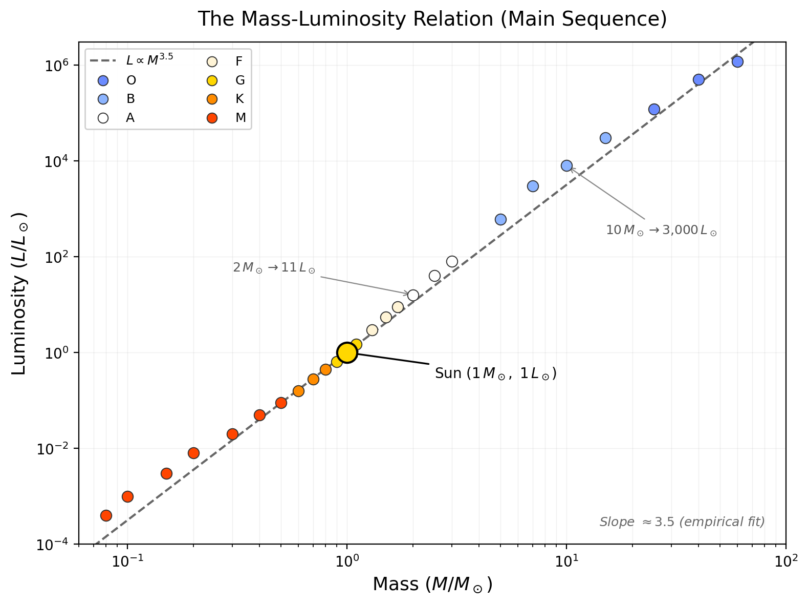
What to notice: along the main sequence, luminosity rises much faster than mass. Small changes in mass produce enormous changes in power output, which is why massive stars burn through their fuel so quickly.
| Mass (\(M_\odot\)) | Luminosity (\(L_\odot\)) | Approximate Main-Sequence Lifetime |
|---|---|---|
| 0.5 | ~0.1 | ~50-100+ Gyr |
| 1.0 | 1 | ~10 Gyr |
| 2.0 | ~10 | ~1-2 Gyr |
| 5.0 | ~300 | ~0.1-0.2 Gyr |
| 10 | ~3000 | ~0.02-0.03 Gyr |
| 20 | ~40000 | a few Myr |
Look at that table. The pattern is unmistakable. Massive stars are stunningly bright — but at a cost.
Main sequence: The band on the Hertzsprung-Russell diagram where stars spend most of their lives, fusing hydrogen into helium in their cores. The mass-luminosity relation applies to main-sequence stars.
This is a main-sequence relation only. Giants, supergiants, and white dwarfs do not follow the same mass-luminosity rule.
Along the main sequence, stellar mass is the hidden physical variable that largely determines where a star sits on the H-R diagram: higher-mass stars are hotter, bluer, and more luminous.
That is why the main sequence is a physical sequence, not just a random band of stars on the H-R diagram.
Why Does This Relationship Exist?
The deeper reason lies in stellar physics. A more massive star has a hotter, denser core. Higher core temperature means hydrogen fuses faster — and stellar fusion rates respond very steeply to temperature, especially in more massive stars where the CNO cycle becomes important. So a \(2 \, M_\odot\) star does not just fuse twice as fast as the Sun. It fuses much faster, making it much more luminous.
A more massive star can support a hotter, denser core because of its higher gravity. The weight of all that overlying material compresses the core to higher pressure and temperature. The more massive the star, the hotter the core must be to support the weight, and the faster fusion occurs.
higher mass
\(\rightarrow\) stronger gravity
\(\rightarrow\) higher core pressure and temperature
\(\rightarrow\) faster fusion
\(\rightarrow\) higher luminosity
If mass increases, which should respond more dramatically: the amount of fuel available or the fusion rate? Explain your reasoning from the causal chain above.
The mass-luminosity relation is not a law we impose; it emerges from stellar structure and the physics of nuclear fusion. A main-sequence star’s luminosity is determined almost entirely by its mass. This is why mass is destiny.
Applying the Mass-Luminosity Relation
We can use the mass-luminosity relation in two directions.
Forward: Given a star’s mass, predict its luminosity.
For a \(3 \, M_\odot\) main-sequence star,
\[ \frac{L}{L_\odot} \approx \left(\frac{3 \, M_\odot}{M_\odot}\right)^{3.5} = 3^{3.5} \approx 46 \]
\[ L \approx 46 \, L_\odot \]
Does this answer make physical sense? Yes. A star only three times the Sun’s mass being dozens of times brighter matches the steep \(M^{3.5}\) scaling.
Backward: Given a star’s luminosity, estimate its mass.
If we observe that a main-sequence star is \(100\) times more luminous than the Sun, then
\[ \frac{100 \, L_\odot}{L_\odot} \approx \left(\frac{M}{M_\odot}\right)^{3.5} \]
\[ 100 \approx \left(\frac{M}{M_\odot}\right)^{3.5} \]
\[ \frac{M}{M_\odot} \approx 100^{1/3.5} \approx 3.98 \]
\[ M \approx 3.98 \, M_\odot \]
This star has a mass of about \(4 \, M_\odot\).
Does this answer make physical sense? Yes. A star around four times the Sun’s mass being about 100 times as luminous is in the right ballpark for the main-sequence relation.
A main-sequence star has a mass of \(2.5 \, M_\odot\). Using the mass-luminosity relation, what is its luminosity relative to the Sun? Show enough reasoning that someone can follow your exponent work.
[Solution] Start with
$$ ()^{3.5} = (2.5)^{3.5}
$$ Rewrite the exponent:
$$ (2.5)^{3.5} = (2.5)^{7/2} = (2.5)^3 (2.5)^{1/2}
$$ Evaluate each part:
$$ (2.5)^3 = 15.625
$$
$$ (2.5)^{1/2} =
$$ Multiply them:
$$
$$ So
$$ L , L_
$$ A \(2.5 \, M_\odot\) main-sequence star is about 25 times more luminous than the Sun.
The mass-luminosity relation makes mass the hidden variable behind main-sequence brightness and H-R diagram position.
Stellar Lifetimes: How Long Does the Fuel Last?
Here is the ultimate consequence of the mass-luminosity relation: massive stars burn out quickly.
Massive stars have more fuel. Why doesn’t that mean they live longer?
A star’s main-sequence lifetime depends on two competing ideas:
- Fuel available \(\propto M\)
- Burn rate \(\propto L\)
- Therefore lifetime \(\propto \frac{M}{L}\)
The first line says a more massive star has more hydrogen available overall. The second says a more luminous star burns through that fuel faster. Lifetime depends on the balance between those two effects.
We can write that balance as
\[ \tau \propto \frac{M}{L} \]
- \(\tau\) = main-sequence lifetime
- \(M\) = stellar mass
- \(L\) = luminosity
- This equation says lifetime depends on fuel divided by burn rate
Now bring in the mass-luminosity relation:
\[ L \propto M^{3.5} \]
- \(L\) = luminosity
- \(M\) = mass
- This is the main-sequence scaling from the previous section
Substitute that into the lifetime relation:
\[ \tau \propto \frac{M}{M^{3.5}} = M^{-2.5} \]
- \(\tau\) = lifetime
- \(M^{-2.5}\) = mass raised to the negative 2.5 power
- This equation returns the scaling of lifetime with mass
For calculations, it is helpful to use the normalized working equation
\[ \frac{\tau}{10 \, \mathrm{Gyr}} \approx \left(\frac{M}{M_\odot}\right)^{-2.5} \]
- \(\tau\) = main-sequence lifetime
- \(10 \, \mathrm{Gyr}\) = the Sun’s approximate total main-sequence lifetime
- \(\frac{M}{M_\odot}\) = mass relative to the Sun
- This equation returns lifetime in units of the Sun’s lifetime
Lifetime is inversely proportional to the 2.5 power of mass. More massive stars live much shorter lives.
Let’s work out some numbers. The Sun has burned hydrogen for about 5 billion years and has about 5 billion years left, for a total hydrogen-burning lifetime of roughly 10 billion years.
For a \(2 \, M_\odot\) star,
\[ \frac{\tau}{10 \, \mathrm{Gyr}} \approx \left(\frac{2 \, M_\odot}{M_\odot}\right)^{-2.5} = 2^{-2.5} \approx \frac{1}{5.66} \]
\[ \tau \approx 10 \, \mathrm{Gyr} \times \frac{1}{5.66} \approx 1.8 \, \mathrm{Gyr} \]
A \(2 \, M_\odot\) star lives roughly 1.8 billion years.
Does this answer make physical sense? Yes. The star has only about twice the fuel, but it shines roughly 10 times more brightly, so it should run out much sooner than the Sun.
A \(10 \, M_\odot\) star is even more extreme:
\[ \frac{\tau}{10 \, \mathrm{Gyr}} \approx \left(\frac{10 \, M_\odot}{M_\odot}\right)^{-2.5} = 10^{-2.5} \approx \frac{1}{316} \]
\[ \tau \approx 10 \, \mathrm{Gyr} \times \frac{1}{316} \approx 0.032 \, \mathrm{Gyr} = 32 \, \mathrm{Myr} \]
A \(10 \, M_\odot\) star lives only about 32 million years.
Does this answer make physical sense? Yes. A very massive star is extraordinarily luminous, so it burns through its fuel on a timescale that is tiny compared with the Sun’s.
If a star cluster is truly old, would you expect it to still contain hot blue high-mass main-sequence stars? Explain what lifetime argument you are using.
| Mass (\(M_\odot\)) | Lifetime |
|---|---|
| 0.5 | ~50-100+ Gyr |
| 1.0 | ~10 Gyr |
| 2.0 | ~1.8 Gyr |
| 5.0 | ~0.1-0.2 Gyr |
| 10 | ~32 Myr |
| 20 | ~5-6 Myr |
The message is stark: massive stars live fast and die young. Very massive stars can exceed \(100 \, M_\odot\), but the simple \(M^{-2.5}\) scaling becomes less reliable at the highest masses. For ASTR 101, treat it as an order-of-magnitude guide to main-sequence lifetimes, not as an exact rule for every star.
Main-sequence lifetime scales roughly as \(\tau \propto M^{-2.5}\). A star 2 times more massive lives roughly 6 times shorter. A 10-times-more-massive star lives roughly 300 times shorter. This is why we see massive stars almost only in young star clusters — they have already burned out in older populations.
This is an approximate main-sequence scaling. Real stellar lifetimes also depend on how much of a star’s mass can actually participate in core fusion and on how stellar structure changes with mass.
“More massive stars should live longer because they have more fuel.” They do have more fuel, but their luminosities rise even faster. The faster burn rate wins.
If the Sun’s lifetime is \(10 \, \mathrm{Gyr}\), what is the lifetime of a \(3 \, M_\odot\) main-sequence star? Then explain in words why the answer is shorter than the Sun’s.
[Solution] Use
$$ ()^{-2.5} = 3^{-2.5}
$$ Then
$$ , ,
$$ So a \(3 \, M_\odot\) star lives about \(0.64 \, \mathrm{Gyr}\), or about 640 million years. The reason is that luminosity rises much faster than the fuel supply, so the star burns through its hydrogen far more quickly than the Sun.
Massive stars die young because luminosity rises much faster than the available fuel supply.
Putting It Together: Mass Is Destiny
This section is the whole lecture in compressed form.
A star’s birth mass determines:
Its position on the main sequence in the H-R diagram. More massive stars are hotter and more luminous.
Its luminosity through the mass-luminosity relation: \(L \propto M^{3.5}\).
Its lifetime through the mass-lifetime relation: \(\tau \propto M^{-2.5}\).
Its later fate. Massive stars cannot quietly fade the way the Sun will.
How we estimate the masses of single stars. Binary systems calibrate the relations that let us infer masses for ordinary main-sequence stars that are not in useful binaries.
\[ \text{birth mass} \rightarrow \text{main-sequence position} \rightarrow \text{luminosity} \rightarrow \text{lifetime} \rightarrow \text{end state} \]
Birth mass sets a star’s place on the main sequence, how bright it shines, how long it lives, and how it ends.
Everything in this reading points back to the same conclusion: for stars, mass is the master variable.
Suppose you observe an old star cluster and find that it still contains hot, blue \(10 \, M_\odot\) main-sequence stars. What would that tell you about the cluster’s age, and why?
[Solution] It would tell you the cluster cannot actually be old. A \(10 \, M_\odot\) main-sequence star lives only about \(30\) million years, so any cluster that still contains such stars must be younger than that order of magnitude.
The exact exponent in the mass-luminosity relation varies somewhat with mass range. For very massive stars the relation is often shallower than \(M^{3.5}\), and for low-mass stars it is often somewhat flatter too. For ASTR 101, the important idea is the broad pattern: more massive main-sequence stars are much more luminous and therefore much shorter-lived.
Deep Dive: The Uncertainty in Measuring Stellar Masses
How confident are we in the masses we measure from binaries? The answer is: very confident for the best systems, but not equally confident for every binary.
Sources of uncertainty:
- Orbital inclination: If the orbit is not edge-on, we may see only a projected velocity. This is why spectroscopic binaries alone often give minimum masses.
- Distance uncertainty: For visual binaries, angular orbit sizes must be converted into AU. If the distance is uncertain, the mass is uncertain.
- Blending: A faint companion can hide in the light of a brighter star, making the spectrum or light curve harder to interpret.
- Non-circular orbits: Real binaries can be elliptical, so the orbital speed changes during the orbit and the full geometry must be modeled carefully.
This is why the best mass measurements often come from systems that are observed in more than one way. Visual information, eclipses, and radial velocities each reduce a different uncertainty.
Deep Dive: Unusual Binaries and Evolution
Some binary systems reveal surprising physics because the stars are at different evolutionary stages.
Algol-type systems: Algol B looks too evolved for its current mass. In a single-star picture, the more massive star should evolve first. The resolution is mass transfer: Algol B used to be the more massive star, evolved more quickly, expanded, and lost mass to Algol A. Today Algol A is more massive, while Algol B is more evolved — a reversal produced by binary interaction.
Common envelope systems: In some close binaries, when one star expands into a giant, it engulfs the other star. The two cores spiral inward inside a shared envelope of gas. If they survive without merging, they can emerge as an extremely close binary.
These systems teach us that binaries are not just measuring tools. They are also laboratories of stellar evolution.
Summary: From Weighing Stars to Understanding Destiny
We have learned how to measure stellar mass and why it matters so much.
Visual binaries: positions on the sky give orbital geometry, and with a distance measurement astronomers can convert the orbit into AU and get the total mass.
Eclipsing binaries: light curves constrain inclination and stellar radii, making the geometry much less ambiguous.
Spectroscopic binaries: Doppler shifts reveal radial velocities and often the mass ratio, but usually give minimum masses unless inclination is known.
Binary mass equation: in solar units,
\[ M_1 + M_2 = \frac{a^3}{P^2} \] with \(a\) in \(\mathrm{AU}\), \(P\) in \(\mathrm{yr}\), and mass in \(M_\odot\).
- Main-sequence scaling laws:
\[ \frac{L}{L_\odot} \approx \left(\frac{M}{M_\odot}\right)^{3.5} \] and
\[ \frac{\tau}{10 \, \mathrm{Gyr}} \approx \left(\frac{M}{M_\odot}\right)^{-2.5} \]
- Mass is destiny: birth mass largely sets a star’s main-sequence position, luminosity, lifetime, and end state.
In Lecture 19, we will trace what happens as a main-sequence star ages. We will see why the Sun gradually brightens over its lifetime and why more massive stars cannot remain stable on the main sequence for long. The mass-lifetime relation is the skeleton key that unlocks stellar evolution.
Practice Problems
Solutions are available in the Lecture 17 Solutions.
Core Problems
Problem 1: A visual binary has an orbital period of 20 years and a separation of 4 AU. What is the combined mass of the two stars in solar masses? Use \(P\) in years and \(a\) in AU.
Problem 2: In a spectroscopic binary, the primary star has a radial velocity amplitude of \(25 \, \mathrm{km\,s^{-1}}\) and the secondary has an amplitude of \(50 \, \mathrm{km\,s^{-1}}\). What is the mass ratio \(M_2 /M_1\)? Explain which star is more massive.
Problem 3: A main-sequence star has a mass of \(4 \, M_\odot\). Using the mass-luminosity relation, how many times more luminous is it than the Sun?
Problem 4: If the Sun’s lifetime is \(10 \, \mathrm{Gyr}\), what is the lifetime of a \(2.5 \, M_\odot\) main-sequence star?
Problem 5: A main-sequence star is observed to be 200 times more luminous than the Sun. Estimate its mass using the mass-luminosity relation.
Problem 6: An eclipsing-binary light curve shows one deep eclipse and one shallower eclipse each orbit. What does that tell you about the two stars, and what extra measurement would you want if your goal were to determine precise stellar masses?
Challenge Problems
Challenge 1: A spectroscopic binary has an orbital period of 5 days, a semi-major axis of \(0.074 \, \mathrm{AU}\), and radial velocity curves showing velocity amplitudes of \(100 \, \mathrm{km\,s^{-1}}\) for the primary and \(60 \, \mathrm{km\,s^{-1}}\) for the secondary. Calculate the individual masses of both stars. Convert the period to years before using the solar-unit form of Kepler’s law.
Challenge 2: A binary star system consists of two equal-mass main-sequence stars, each with a mass of \(2 \, M_\odot\). How many times more luminous are the two stars combined compared to the Sun? Use the mass-luminosity relation for each star separately, then add.
Challenge 3: Sirius A (mass \(\approx 2.0 \, M_\odot\), luminosity \(\approx 26 \, L_\odot\)) and Sirius B (mass \(\approx 1.0 \, M_\odot\)) together demonstrate why the mass-luminosity relation is not universal. Sirius B is a white dwarf, not a main-sequence star. Why should we not expect Sirius B to follow the main-sequence mass-luminosity relation?
Challenge 4: Why are binary-star mass measurements foundational for estimating the masses of single main-sequence stars? Answer by connecting binary measurements to the calibration of the mass-luminosity relation.
Glossary
- ★ Binary star system
- Two stars orbiting a shared center of mass under mutual gravity.
- ★ Center of mass
- The point that two orbiting objects both orbit. Located closer to the more massive object.
- ★ Eclipsing binary
- A binary system oriented edge-on, so one star periodically passes in front of the other, dimming the total light.
- ★ Kepler's third law (Newton's form)
- \(M_1 + M_2 = \frac{a^3}{P^2}\) (in solar units). Relates orbital period and separation to the total mass of a binary.
- ★ Main sequence
- The band on the H-R diagram where stars spend ~90% of their lives fusing hydrogen to helium. The mass-luminosity relation applies here.
- ★ Mass transfer
- The process by which material flows from one star to another in a binary system, often during the red giant phase.
- ★ Mass-luminosity relation
- The empirical relationship for main-sequence stars: \(L \propto M^{3.5}\).
- ★ Orbital period
- The time it takes for two stars to complete one full orbit around their center of mass.
- ★ Radial velocity
- The component of motion toward or away from the observer, measured via Doppler shift.
- ★ Roche lobe
- The region of space around a star where its gravity dominates. If one star expands beyond its Roche lobe, mass can transfer to its companion.
- ★ Semi-major axis
- The long axis of an elliptical orbit, or equivalently, the average separation for a circular orbit.
- ★ Spectroscopic binary
- A binary system detected through Doppler shifts in stellar spectra as the stars orbit. Often too close to resolve visually.
- ★ Visual binary
- A binary system where both stars are bright and far apart enough to resolve as separate objects.
- ★ White dwarf
- A stellar remnant (the core of a dead star) about the size of Earth but with roughly the mass of the Sun. Sirius B is a classic example. Algol B is not a white dwarf; it is an evolved star in a mass-transfer binary.