Lecture 23: The Galaxy Zoo
Classifying Galaxies, Meeting Quasars, and Previewing the Cosmic Web
The Big Idea
The Milky Way is not special because it is the only galaxy. It is special because it is the galaxy we can study from the inside.
Once we look beyond the Milky Way, astronomy becomes a classification-and-inference problem. Galaxies come in recognizable shapes, but those shapes are not just labels. They are clues.
Observable: Galaxies have different shapes, colors, gas contents, spectra, central activity, and clustering patterns.
Model: Stars, gas, dust, black-hole accretion, gravity, and dark matter connect those observables to physical histories.
Inference: A galaxy image is not just a picture. It is evidence for star formation, gas supply, mergers, central black-hole growth, and the large-scale structure of the universe.
This lecture is about learning to read galaxies as evidence.
- Galaxy shapes tell us about stars, gas, and recent history.
- Galaxy distances tell us how big, bright, and massive galaxies really are.
- Active galactic nuclei reveal feeding supermassive black holes.
- Galaxy maps reveal the cosmic web traced by dark matter.
This page answers four questions:
- What kinds of galaxies are there, and what do their shapes tell us?
- Why is measuring galaxy distances hard?
- What are quasars, and why are they not stars?
- How are galaxies arranged on the largest scales?
Punchline: Galaxy morphology is a stellar-population clue. Quasars are accretion signatures from supermassive black holes. The cosmic web is the large-scale pattern of matter, with galaxies acting as the visible tracers.
Focus less on memorizing names and more on the reasoning pattern:
What do we observe?
What physical model explains it?
What can we infer from that model?
Before you settle into the reading, open Rubin’s Tour of Galaxies. Treat it like a first-pass observing exercise: choose a few galaxies, describe what you notice about their shapes and colors, then ask what physical histories those appearances might imply.
If you are short on time, focus on:
- the Hubble Sequence section,
- the Distance Problem section,
- the Active Galactic Nuclei section,
- the Cosmic Web section.
After 20 minutes, you should be able to classify the three main galaxy types, explain what a quasar is, and describe why distances are essential for turning galaxy images into physical knowledge.

What to notice: Module 3 uses the same evidence chain over and over. Dust, 21-cm emission, S-star orbits, galaxy shapes, Cepheid periods, supernova brightness, redshifts, AGN jets, CMB anisotropies, and light-element abundances become physical claims only after a model translates them. (Credit: Illustration: A. Rosen (SVG))
The same reasoning loop appears across the module. Observables become physical claims only after a model connects light, motion, and distance to real properties.
Learning Outcomes
By the end of this reading, you should be able to say:
- I can classify a galaxy as elliptical, spiral, barred spiral, or irregular from an image.
- I can connect a galaxy’s color and structure to its stellar population, gas content, and star-formation activity.
- I can explain why apparent brightness alone does not tell us distance.
- I can describe why standard candles are needed to measure distances beyond the Milky Way.
- I can explain what an active galactic nucleus is and why its energy comes from accretion, not fusion.
- I can describe the basic evidence for a connection between supermassive black holes and their host galaxies.
- I can explain what the cosmic web is and why galaxies trace the underlying dark-matter distribution.
Beyond the Milky Way
Lecture 22 ended at the Galactic Center, about \(8\ {\rm kpc}\) from Earth. Now we step outward.
At about \(50\ {\rm kpc}\), we reach the Large Magellanic Cloud, a small companion galaxy of the Milky Way. At about \(780\ {\rm kpc}\), or about \(2.5\) million light-years, we reach Andromeda, the nearest large spiral galaxy.
Beyond that, the universe opens into a population of galaxies. The exact number of galaxies in the observable universe is not a directly counted fact. It depends on how we model the faintest galaxies that current telescopes cannot individually detect. A safe ASTR 101 statement is:
The observable universe contains at least hundreds of billions of galaxies, and possibly more depending on how many faint galaxies exist below current detection limits.
Observable: Deep images show thousands of galaxies in tiny patches of sky.
Model: We estimate how many faint galaxies are missed by the image.
Inference: The observable universe contains an enormous galaxy population, but the exact number depends on the model for faint galaxies.
The Local Group is the first place where the word “galaxy” stops meaning only “the Milky Way” and starts meaning a population. It contains a few large galaxies, several intermediate companions, and many dwarf galaxies whose faintness makes them hard to census completely.
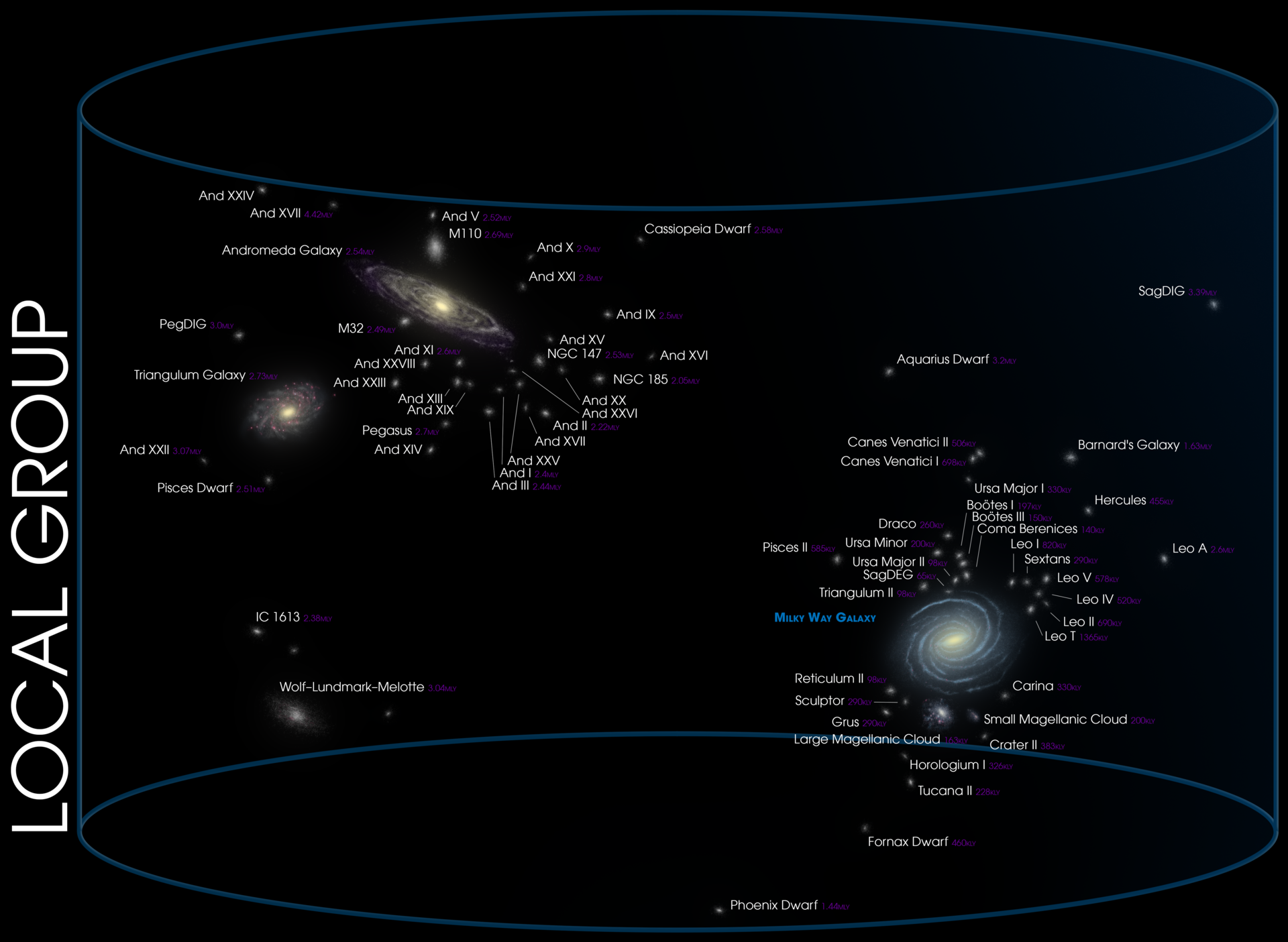
What to notice: the Milky Way is one member of a small gravitational neighborhood. Andromeda, Triangulum, the Magellanic Clouds, and many dwarf galaxies together make up the Local Group. (Credit: Course-provided figure)
The Local Group is not one galaxy plus empty space. It is a gravitational neighborhood, with the Milky Way, Andromeda, Triangulum, the Magellanic Clouds, and many faint dwarf galaxies.
Andromeda is the nearest large spiral in that neighborhood. Because it is close enough for Hubble to resolve individual stars across its disk, it lets us connect the stellar-population tools from Module 2 to the galaxy-scale questions of Module 3.
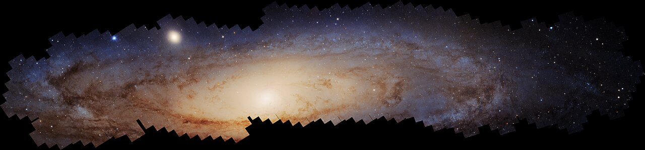
What to notice: Andromeda is close enough for Hubble to resolve enormous numbers of individual stars. That makes it both a neighboring galaxy and a bridge between stellar astronomy and galaxy astronomy. (Credit: NASA/ESA/Hubble)
Andromeda is a galaxy, but it is also a resolved stellar population. Its disk, dust lanes, blue star-forming regions, and older bulge show how galaxy morphology is built from stars and gas.
Before we jump to deep fields, pause on the nearby universe. The Local Group is not a representative sample of all galaxies, but it is the place where distances, sizes, and morphology are easiest to compare directly.
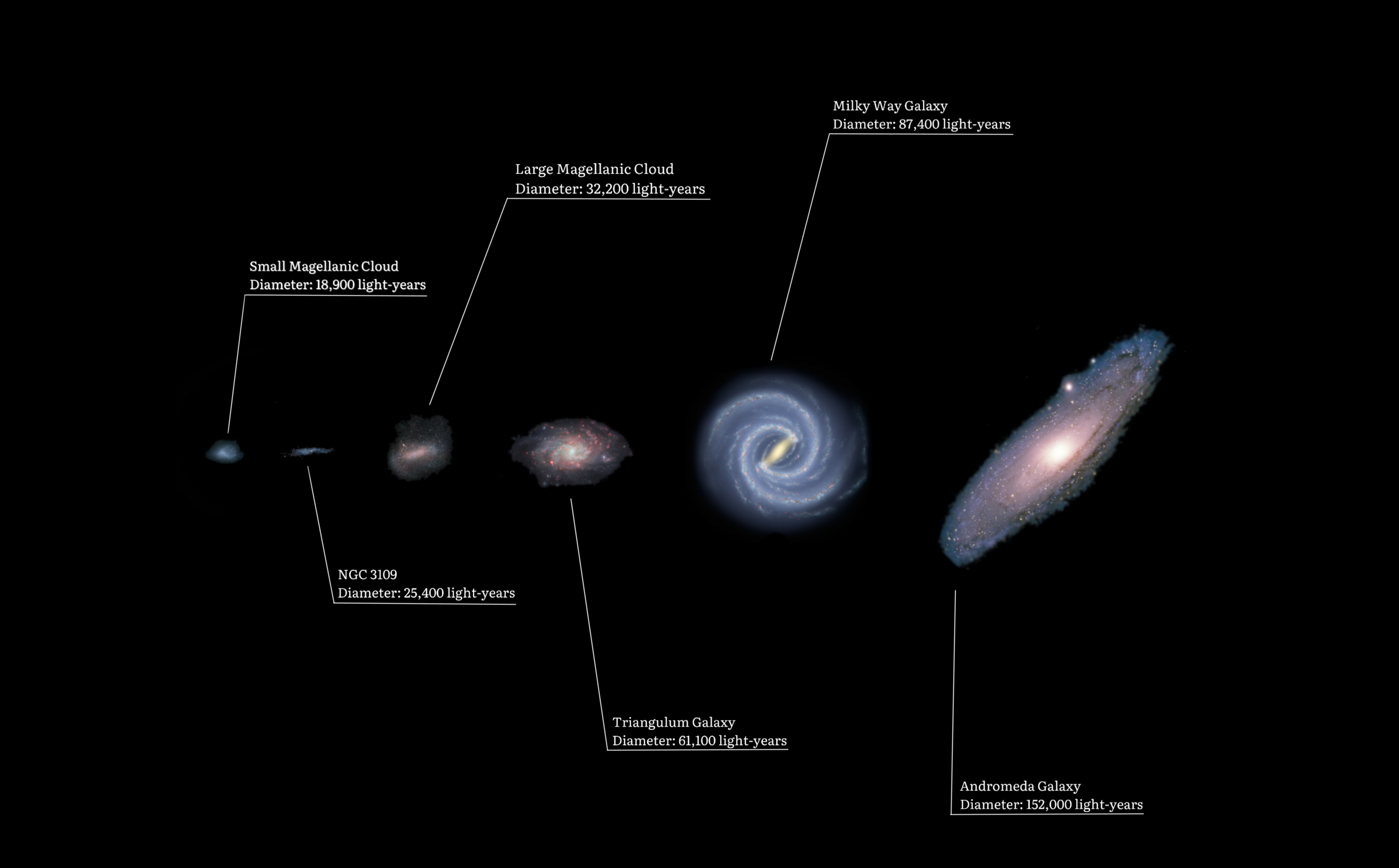
What to notice: the Local Group contains a few large galaxies and many much smaller companions. Galaxy size varies enormously even before we leave our own neighborhood. (Credit: Course-provided figure)
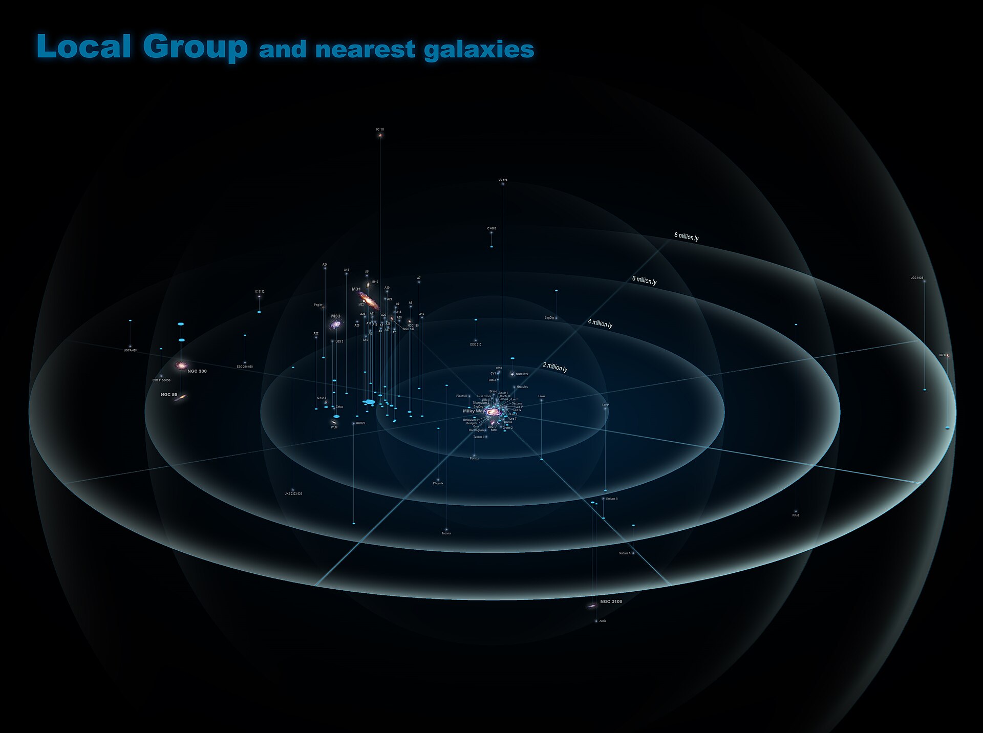
What to notice: the Local Group is the nearby knot in a larger galactic neighborhood. The next galaxies are already millions of light-years away, so distance changes the scale of the story quickly. (Credit: Course-provided figure)
Galaxy size and galaxy spacing are different ideas. The Local Group contains a few large galaxies and many small companions spread across millions of light-years.
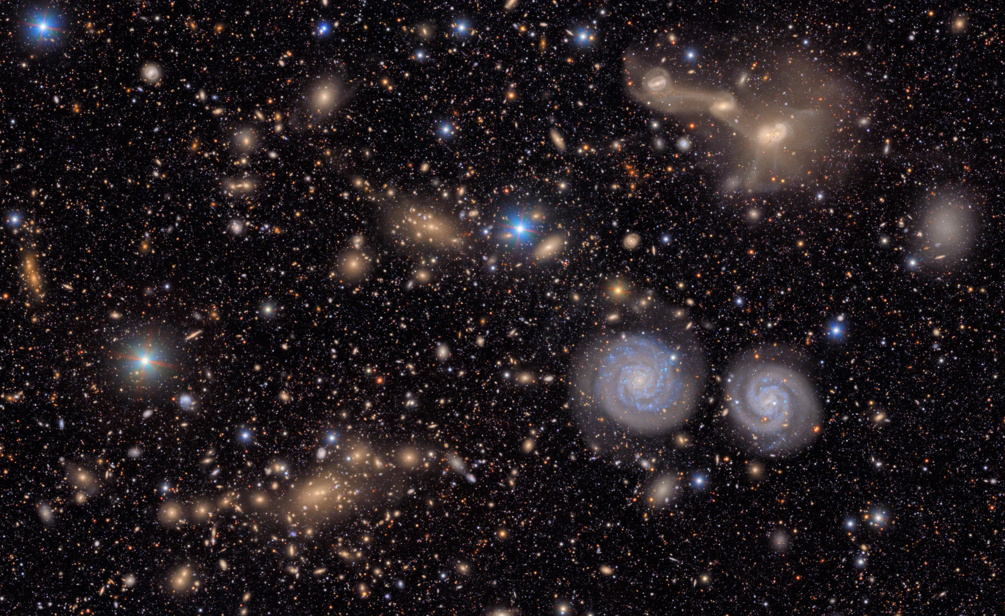
What to notice: a deep survey image is a population sample. Each galaxy is both an object with a morphology and a distance marker waiting for the ladder to place it in three-dimensional space. (Credit: Rubin Observatory/NSF/AURA)
A deep survey field is already a population sample. Each small galaxy-like smudge has a morphology, a color, and a distance that must be inferred.

What to notice: nearly every tiny smudge is a galaxy. A deep field turns an apparently empty patch of sky into evidence for a universe filled with galaxies at many distances and lookback times. (Credit: NASA/ESA/Hubble)
Nearly every faint smudge is a galaxy. The image turns apparently empty sky into evidence for a universe filled with galaxies at many distances and lookback times.
Use the exposure-time slider to watch a dark patch of sky turn into a field of galaxies. Start at the shortest exposure and ask: which specks would you trust as real? Then move right and notice how repeated exposures separate faint sources from noise.
What to notice: “empty sky” is often an exposure-time statement, not a physical statement. Deep fields are why we know the galaxy population includes faint, distant systems whose light has been traveling for most of cosmic history.
Deep-field galaxies are also multiwavelength objects. A galaxy that looks like a faint blob in visible light may reveal hidden star formation at radio wavelengths, where dust is less of an obstacle.
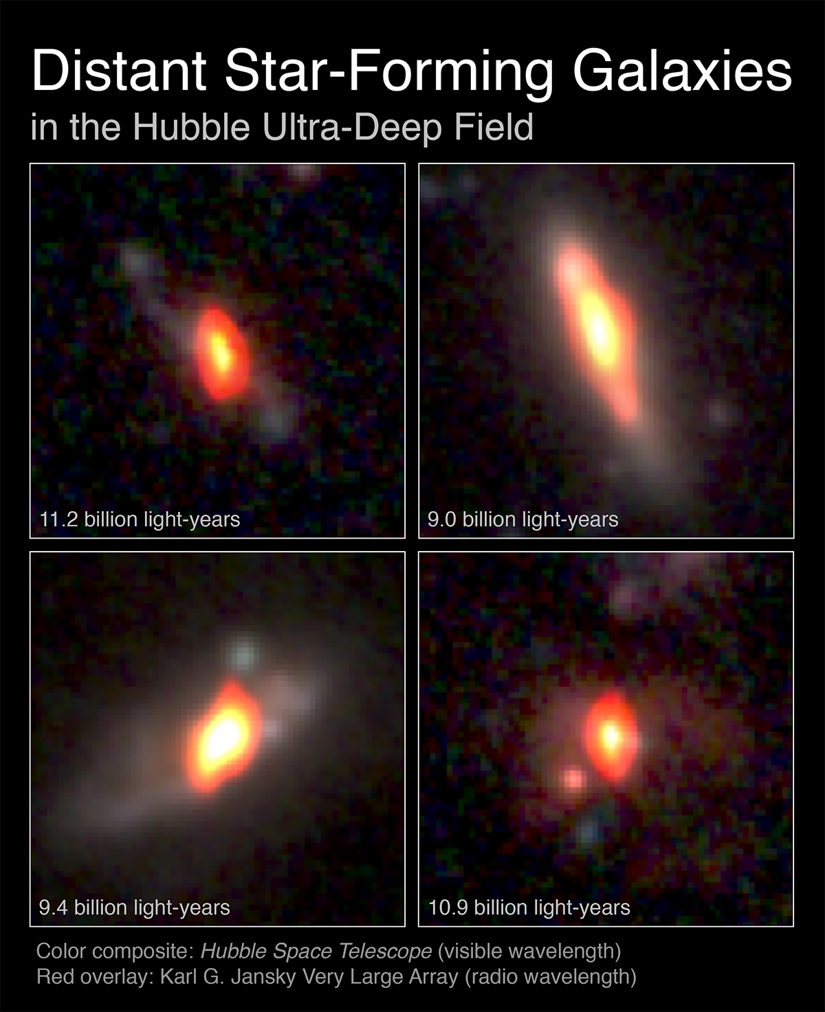
What to notice: distant galaxies are often multiwavelength measurements, not simple photographs. Visible light shows the stellar body, while radio emission can flag dust-obscured star formation. (Credit: Hubble Space Telescope and Karl G. Jansky Very Large Array)
Visible light and radio light can reveal different parts of the same galaxy. The physical inference depends on wavelength: stars, dust, gas, and star formation do not all advertise themselves in the same band.
What you would notice looking at those galaxies is that they are not random. Most of them fall into a small number of shape categories that were first systematized by Edwin Hubble in 1926: the so-called Hubble sequence, or Hubble tuning fork.
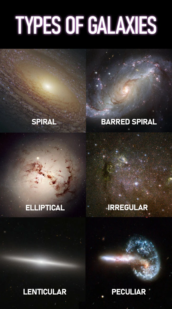
What to notice: these labels are visual starting points. A galaxy’s type is a clue about stars, gas, dust, and interaction history, not a complete biography by itself. (Credit: Course-provided figure)
The visual categories are starting points. A galaxy’s type is a clue about stars, gas, dust, and interaction history, not a complete biography.
The Hubble Sequence
Galaxies come in a few broad visual categories. This classification system is called the Hubble sequence.
The important idea is not that galaxies have names. The important idea is that appearance is evidence.
A galaxy’s shape, color, dust, gas, and star-forming regions help us infer its physical state.
The three main galaxy families
Elliptical galaxies are smooth, rounded or football-shaped systems. They are usually dominated by older, redder stars and contain relatively little cold gas and dust. Because cold gas is the raw material for star formation, most ellipticals have little ongoing star formation.
Spiral galaxies have disks, central bulges, and spiral arms. Their arms often contain gas, dust, young blue stars, and pink H II regions. These are signs of ongoing star formation. The Milky Way is a barred spiral.
Irregular galaxies do not have a clean spiral or elliptical shape. Many are small, gas-rich, and actively forming stars. Some look irregular because gravitational interactions have disturbed them.
The Hubble tuning fork is a classification diagram, not a life cycle.
Ellipticals do not automatically turn into spirals, and spirals do not simply move along the fork from one subtype to another. A galaxy’s type can change through mergers, gas loss, gas accretion, and changes in star formation.
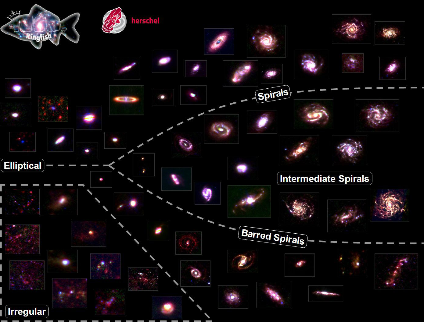
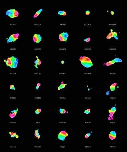
What to notice: the Hubble tuning fork is a classification map, not an evolutionary conveyor belt. The images here are infrared views of dust in nearby galaxies, so morphology is being connected to interstellar material and star formation. (Credit: C. North, M. Galametz & the KINGFISH Team)
The diagram sorts galaxies by appearance. To turn appearance into physics, ask:
- Is there a disk?
- Are there spiral arms?
- Is there dust or gas?
- Are there blue stars or pink H II regions?
- Is the galaxy smooth, red, and mostly featureless?
Galaxy morphology as physical evidence
| Type | What it looks like | Typical stellar population | Gas and dust | Star formation |
|---|---|---|---|---|
| Elliptical | Smooth, round to elongated | Mostly old, red stars | Little cold gas | Usually low |
| Spiral / barred spiral | Disk, bulge, arms, sometimes a bar | Old bulge stars plus young disk stars | Organized gas and dust | Ongoing, especially in arms |
| Irregular | No clean symmetry | Often young and blue | Often gas-rich | Often active or bursty |
A better mnemonic is:
Ellipticals are usually gas-poor. Spirals are still building stars. Irregulars are often dynamically messy.
This is less catchy than “ellipticals are done,” but it is more scientifically honest.
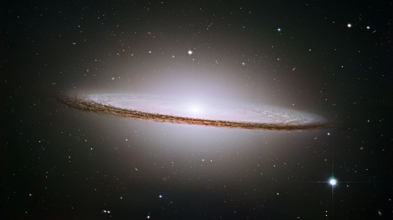
What to notice: the Sombrero Galaxy mixes a bright bulge with a thin dust-rich disk. Real galaxies often sit between tidy textbook categories, so classification is a starting point for physical interpretation. (Credit: NASA/ESA/Hubble)
The Sombrero Galaxy does not fit a cartoon category perfectly. Its bright bulge and thin dusty disk are a reminder that classification is a first inference, not the whole physical story.
Use this as a corrective to the tempting but wrong idea that galaxy type is a fixed identity. Follow the projected Milky Way-Andromeda interaction from separate spirals to a merged elliptical-like remnant.
What to notice: the stars mostly pass by one another, but the gas does not. Gas compression triggers star formation, and later gas depletion helps leave behind a more mature, less star-forming system.
Deep Dive: Galaxy Interactions as Morphology in Motion
The Hubble sequence is a snapshot. Interacting galaxies show why snapshots are not the same as histories.
The Whirlpool Galaxy is a concrete example. Its spiral structure and companion are not independent facts; the interaction helps shape the very pattern we classify.
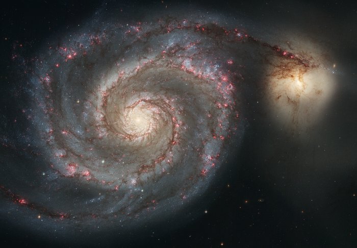
What to notice: the Whirlpool Galaxy turns interaction into structure. Its companion helps organize spiral arms, dust lanes, and star-forming regions, reminding us that morphology records environment. (Credit: NASA/ESA/Hubble)
The companion, spiral arms, dust lanes, and pink star-forming regions belong to one dynamical story. The observable shape is evidence for gravitational interaction.
NGC 602 is a star-forming region in the Small Magellanic Cloud, a satellite galaxy of the Milky Way. Use the exposure-time slider to connect two ideas at once: longer exposures reveal fainter structure, and young massive stars sculpt the gas around them.
What to notice: the same image is both a galaxy-population clue and a stellar-lifecycle clue. The blue young stars, glowing gas, and dusty pillars are the local evidence behind the phrase “gas-rich galaxies are still forming stars.”
M82 pushes the same idea into the extreme. It is a starburst galaxy: gas is being converted into stars so rapidly that feedback from massive stars and supernovae drives material out of the disk.
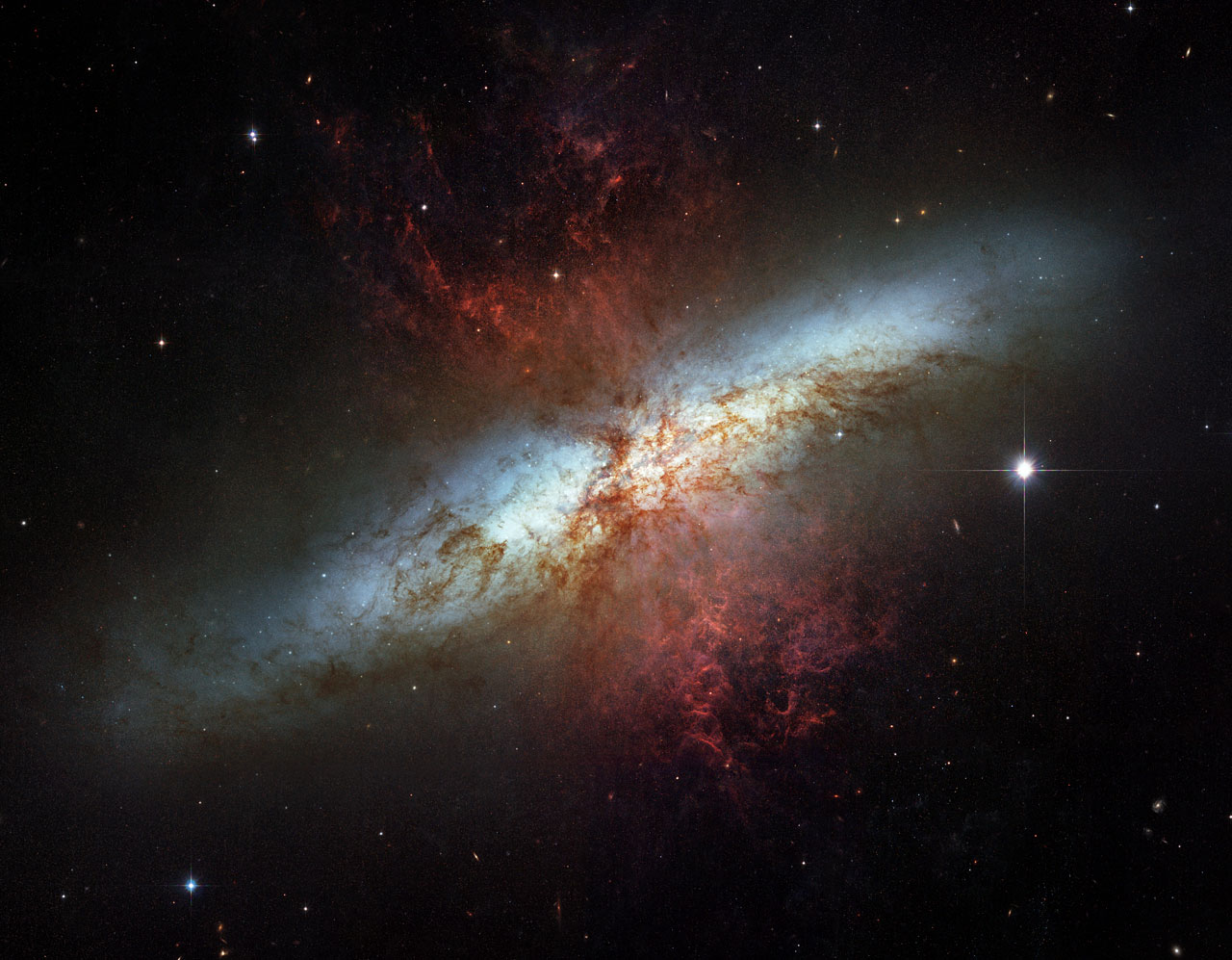
What to notice: starburst galaxies convert gas into stars at an extreme rate. The red outflowing material in M82 is feedback: young massive stars and supernovae pushing gas out of the galaxy. (Credit: NASA/ESA/Hubble)
The red outflow is feedback made visible. Massive stars and supernovae are pushing gas out of the galaxy, so morphology is tied to star formation and gas motion.
Use the wavelength buttons to inspect a real galaxy collision in radio, infrared, visible, and X-ray light. This is a better mental model for galaxy evolution than a static tuning fork.
What to notice: different wavelengths reveal different stages of the same physical event. Radio and infrared trace gas and dust; visible light traces stars and star-forming regions; X-rays reveal compact remnants and hot gas from earlier waves of massive-star evolution.
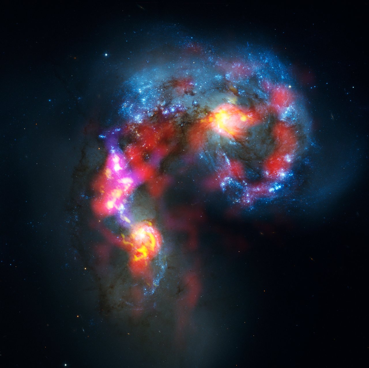
What to notice: the Antennae collision is both a stellar event and a gas event. Blue starlight shows young populations, while the radio and submillimeter gas overlay marks where compressed material can fuel new star formation. (Credit: ESO/ALMA/Hubble)
The Antennae collision is both a stellar event and a gas event. The blue starlight and gas overlay reveal where the merger is compressing material and triggering star formation.
Galaxy interactions are not just visual distortions in starlight. They also move the cold molecular gas that will make the next generation of stars. In a merger, the gas can be driven into the center, pulled into tidal features, or compressed into off-center star-forming knots.
What to notice: galaxy interactions rearrange cold molecular gas in many different ways. The gas distribution is the clue to where future star formation can be triggered, suppressed, or concentrated. (Credit: Course-provided figure)
The gas maps show where future stars can form. In mergers, cold molecular gas can be concentrated, displaced, stretched, or compressed, so the next generation of stars is written into the gas distribution before it appears in starlight.
You observe two galaxies.
Galaxy A is a smooth red ellipsoid with almost no cold gas detected at 21 cm.
Galaxy B is a blue-tinged pinwheel with pink H II regions along its arms.
Before reading the answer, predict:
- Which galaxy is forming stars today?
- Which galaxy has the older average stellar population?
- What observable clues support your answer?
Galaxy B is forming stars today.
The key clues are the blue color and the pink H II regions. Blue light often comes from young, hot, massive stars. H II regions are clouds of ionized hydrogen around young massive stars, so they are direct evidence of recent star formation.
Galaxy A has the older average stellar population. Its red color, smooth structure, and lack of cold gas suggest that it is dominated by older stars and has little raw material available for new star formation.
This is the Module 2 H-R diagram applied at the scale of an entire galaxy.
The Distance Problem
Classifying a galaxy from an image is the easy part. The harder question is:
How far away is it?
Distance matters because the sky gives us apparent properties, but astronomy often needs physical properties.
A galaxy that looks faint could be:
- nearby and intrinsically dim, or
- far away and intrinsically bright.
A galaxy that looks small could be:
- physically small, or
- physically large but far away.
Without distance, we cannot reliably convert apparent brightness into luminosity, apparent size into physical size, or observed motion into mass.
A bright object is not necessarily nearby, and a faint object is not necessarily far away.
Brightness on the sky depends on both intrinsic luminosity and distance.
For stars, parallax gives direct distances nearby. But parallax becomes too small to measure for most extragalactic objects. Andromeda is about \(780\ {\rm kpc}\) away, far beyond the range where ordinary stellar parallax can map the galaxy as a whole.
So astronomers use standard candles.
A standard candle is an object whose true luminosity \(L\) can be estimated from its physics. If we know \(L\) and measure the received flux \(F\), then the inverse-square law gives the distance.
\[ F = \frac{L}{4\pi d^2} \]
Solving for distance gives:
\[ d = \sqrt{\frac{L}{4\pi F}} \]
where:
- \(F\) is the measured flux at Earth, in \({\rm W\,m^{-2}}\),
- \(L\) is the object’s intrinsic luminosity, in \({\rm W}\),
- \(d\) is the distance to the object, in \({\rm m}\) if SI units are used.
Light spreads out as it travels. At twice the distance, the same light is spread over four times the area. That is why flux decreases as \(1/d^2\).
The quantity \(L/F\) has units:
\[ \frac{{\rm W}}{{\rm W\,m^{-2}}} = {\rm m^2} \]
The square root therefore has units of meters, which is what a distance should have.
For galaxies, the key standard candles are stellar objects:
- Cepheid variables: pulsating stars whose pulsation period tells us their luminosity.
- Type Ia supernovae: exploding white dwarfs with calibratable peak luminosities.
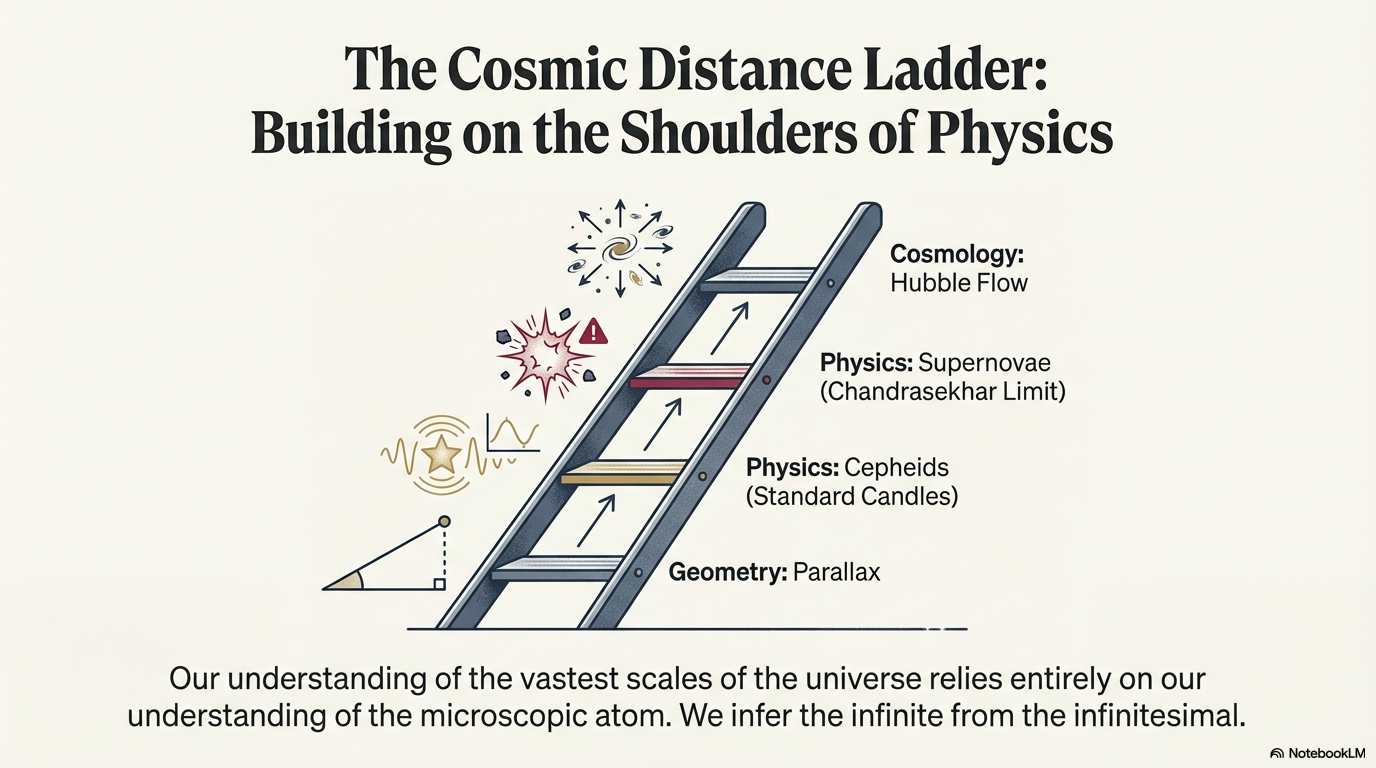
What to notice: Each rung calibrates the next. Parallax (geometry) → Cepheids (standard candles) → Supernovae (Chandrasekhar limit) → Hubble Flow (cosmology). We infer the infinite from the infinitesimal. (Credit: (A. Rosen/NotebookLM))
The distance ladder is built rung by rung. Nearby geometric distances calibrate stellar tools, and those stellar tools eventually calibrate galaxy distances.
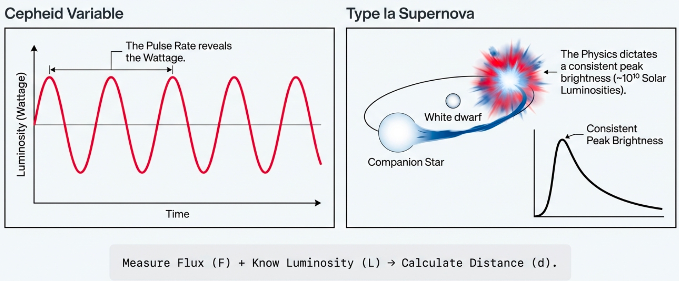
What to notice: Standard candles work because physics predicts their luminosity. Measure flux (F) + know luminosity (L) → calculate distance (d). (Credit: (A. Rosen/NotebookLM))
Standard candles are not “standard” because they all look equally bright from Earth. They are useful because their intrinsic luminosities can be calibrated, letting measured flux become distance.
This is the central lesson of the distance ladder:
Stars are the tools we use to measure the scale of the universe.
A standard candle must have a reliable luminosity \(L\).
Suppose two objects look like the same kind of standard candle, but one is actually \(4\) times more luminous than the other.
Predict before reading:
- If you assumed the wrong luminosity, would the distance error be a factor of \(4\)?
- Or would it be smaller than that?
- Why?
The distance error would be a factor of \(2\), not \(4\).
The distance formula is:
\[ d = \sqrt{\frac{L}{4\pi F}} \]
Distance depends on the square root of luminosity. So if the luminosity is wrong by a factor of \(4\), the distance is wrong by:
\[ \sqrt{4} = 2 \]
This is why standard candles must be reliable. If their luminosities vary too much, every distance estimate becomes uncertain.
Active Galactic Nuclei
Lecture 22 ended with a supermassive black hole at the center of the Milky Way: Sagittarius A*, with a mass of about \(4 \times 10^6\ M_\odot\).
Sagittarius A* is mostly quiet today. It is massive, but it is not currently feeding rapidly.
In some galaxies, the central supermassive black hole is actively accreting gas. As gas spirals inward, it forms a hot accretion disk and releases enormous energy. The bright central region is called an active galactic nucleus, or AGN.
The most luminous AGN are called quasars.
A quasar is not a star.
It is the bright central engine of a galaxy, powered by gas falling toward a supermassive black hole.
What to notice: a quasar is an accretion engine, not a star. The bright disk and jets are powered by gravitational energy released near a supermassive black hole. (Credit: Course-provided figure)
The galaxy can be tens of thousands of light-years across, but the main power source is concentrated near the center. That compactness is one of the clues that the source is not ordinary starlight.
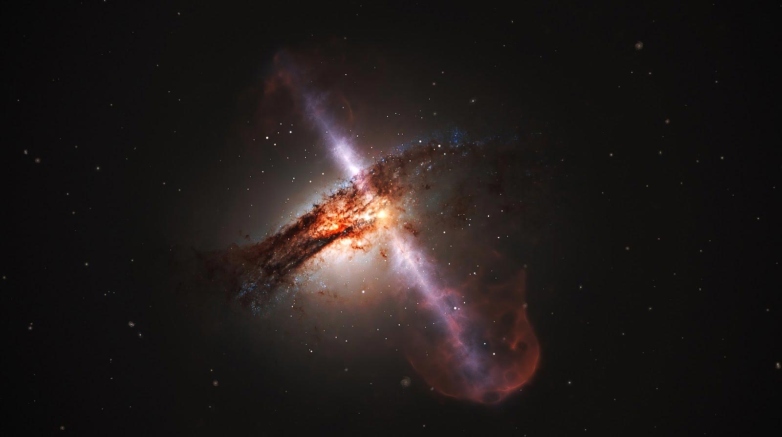
What to notice: an active nucleus is embedded inside a host galaxy. Dust can hide the central engine in some directions while jets carry energy far beyond the black hole’s immediate surroundings. (Credit: ESO)
An active nucleus is embedded inside a host galaxy. Dust can hide the central engine from some viewing angles while jets and outflows carry energy outward.
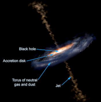
What to notice: the AGN engine is compact. A black hole plus accretion disk sits inside a dusty torus, and some systems launch jets perpendicular to the disk. (Credit: Course-provided figure)
This schematic separates the central engine into parts: black hole, accretion disk, dusty torus, and sometimes jets. Each part leaves different observational signatures.
This schematic is useful as a vocabulary map. Read it with one caution: the event horizon, disk, photon sphere, and jets are physically meaningful regions, while the singularity marks where our classical theory stops being enough.
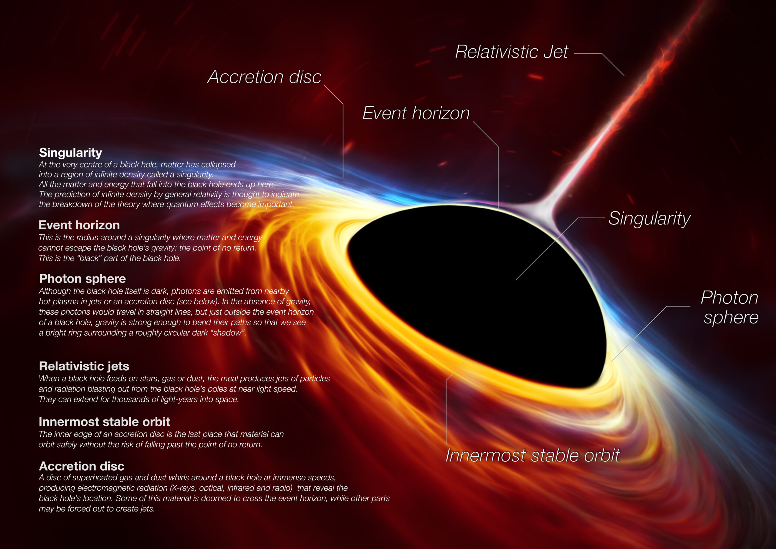
What to notice: the event horizon, accretion disk, photon sphere, and jets are different physical regions. The singularity label is a signpost for where classical general relativity reaches its limit, not something directly observed. (Credit: ESO)
The schematic is a vocabulary map, not a scale drawing. Use it to identify which physical regions produce different signals: disk emission, dust absorption, and jets.
If visible light shows mostly stars, which wavelength would you expect to be more useful for detecting jets from an active galactic nucleus: radio, infrared, or visible? Explain your reasoning before opening the interactive.
Use the wavelength buttons to build a multiwavelength picture of an active galaxy. First look in visible light and ask what is hidden; then compare radio, infrared, and X-ray views.
What to notice: the active SMBH is not just a bright point. Radio and X-ray light reveal jets tens of thousands of light-years long, while infrared and visible light reveal dust and stars from a merger history. This is the AGN engine embedded in a real galaxy.
The same lesson shows up in Hercules A. In visible light, the host galaxy does not announce the scale of the engine. Radio and X-ray views reveal the enormous structures inflated by the active nucleus.
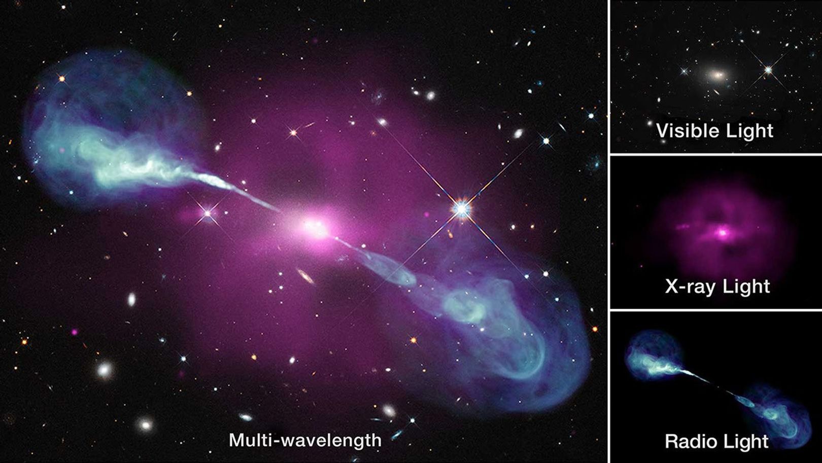
What to notice: visible light alone makes Hercules A look fairly ordinary, but radio and X-ray views reveal enormous jets and lobes powered by the central AGN. (Credit: NASA, ESA, NRAO, and STScI)
The radio structure extends far beyond the visible galaxy. That is why multiwavelength evidence is essential for recognizing AGN jets.
An AGN has four useful components:
- Supermassive black hole: the central compact object, usually millions to billions of solar masses.
- Accretion disk: hot gas spiraling inward and radiating strongly, especially in ultraviolet and X-ray light.
- Dusty torus: colder gas and dust around the central disk, which can hide the engine from some viewing angles.
- Jets: in some AGN, narrow streams of fast-moving plasma launched away from the central region.
An active black hole is bright only when gas is available to fall inward. A supermassive black hole can be massive but quiet if it is not being fed.
Where the Light Comes From
The energy source of a quasar is not nuclear fusion.
Stars shine because fusion converts a small fraction of mass into energy. Hydrogen fusion converts about \(0.7\%\) of the fuel’s rest-mass energy into light.
Quasars shine because of accretion. Gas falling toward a black hole loses gravitational potential energy. In the accretion disk, that energy becomes heat and radiation.
For black-hole accretion, the efficiency can be much higher than fusion:
- hydrogen fusion: about \(0.7\%\) efficient,
- accretion onto a non-rotating black hole: about \(6\%\) efficient,
- accretion onto a rapidly rotating black hole: up to tens of percent efficient.
The exact efficiency depends on black-hole spin and accretion-disk physics, but the ASTR 101 takeaway is simple:
Accretion can release far more energy per kilogram of fuel than fusion.
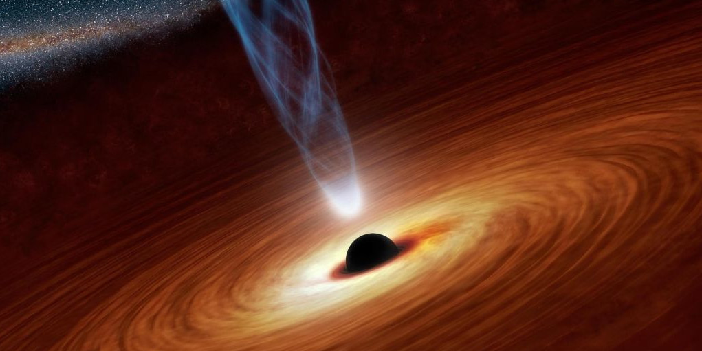
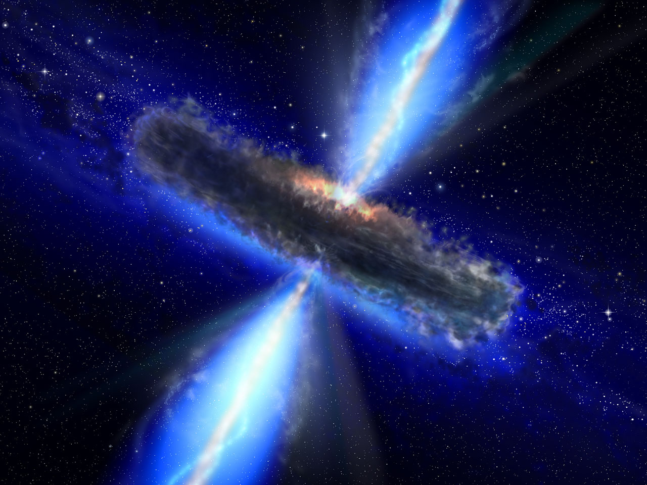
What to notice: the light source is not fusion in stars. Gas releases gravitational energy as it spirals through a hot accretion disk close to a supermassive black hole. (Credit: NASA/JPL-Caltech)
The bright source is the hot accretion flow near the black hole. The energy source is gravitational infall, not nuclear burning in stars.
That is why a quasar can outshine an entire galaxy of stars from a region only light-hours to light-days across.
Quasars can vary in brightness over hours to days.
That matters because no object can change brightness coherently faster than light can cross it. If a quasar changes noticeably in one day, then the region producing that change cannot be much larger than one light-day across.
Before reading the answer, predict:
- Why does rapid variability imply a compact source?
- Why is a compact, extremely luminous source hard to explain with ordinary stars?
- Why does accretion onto a supermassive black hole solve the problem?
Rapid variability means the emitting region must be compact. If different parts of the region were separated by many light-days, they could not coordinate a brightness change in only hours or days.
A dense cluster of ordinary stars cannot easily explain this. Fusion is not efficient enough, and packing enough stars into such a small region would create an unstable system.
Accretion onto a supermassive black hole solves both problems. It is compact, because the energy is released close to the black hole, and it is efficient, because falling gas can convert a large fraction of gravitational energy into radiation.
The Eddington Limit
A feeding black hole cannot increase its luminosity without limit.
As gas falls inward, it releases energy. That radiation pushes outward on the surrounding gas. If the radiation pressure becomes strong enough, it can push gas away and reduce the inflow.
The luminosity where outward radiation pressure balances inward gravity is called the Eddington luminosity.
For ionized gas around a black hole, the approximate scaling is:
\[ L_{\rm Edd} \approx 1.3 \times 10^{31}\ {\rm W}\left(\frac{M}{M_\odot}\right) \]
The important part is the scaling:
\[ L_{\rm Edd} \propto M \]
A more massive black hole has stronger gravity, so it can support a higher accretion luminosity before radiation pressure pushes the gas away.
If we observe an extremely luminous quasar, the Eddington limit gives a minimum black-hole mass. The brightness alone tells us the black hole must be very massive.
Worked Example: Minimum SMBH Mass from Eddington
Suppose a quasar has luminosity:
\[ L \approx 10^{40}\ {\rm W} \]
Use the Eddington scaling:
\[ L_{\rm Edd} \approx 1.3 \times 10^{31}\ {\rm W}\left(\frac{M}{M_\odot}\right) \]
For the quasar to shine at this luminosity without radiation pressure shutting off the inflow, we need:
\[ L \lesssim L_{\rm Edd} \]
So the black hole mass must satisfy:
\[ \frac{M}{M_\odot} \gtrsim \frac{10^{40}\ {\rm W}}{1.3 \times 10^{31}\ {\rm W}} \]
The units cancel, leaving:
\[ \frac{M}{M_\odot} \gtrsim 7.7 \times 10^8 \]
So:
\[ M \gtrsim 8 \times 10^8\ M_\odot \]
Interpretation: A quasar with luminosity \(10^{40}\ {\rm W}\) requires a black hole of roughly a billion solar masses if it is radiating near the Eddington limit.
This is a lower-limit argument. It does not measure the black-hole mass exactly. It says the black hole must be massive enough for gravity to hold onto gas against the outward push of radiation.
The SMBH-Galaxy Connection
Supermassive black holes live in galaxy centers. But they do not grow in isolation.
A major observational clue is that the mass of a galaxy’s central supermassive black hole is correlated with the random speeds of stars in the galaxy’s central bulge. This is called the \(M\)-\(\sigma\) relation.
Here:
- \(M\) means the mass of the central black hole.
- \(\sigma\) means the velocity dispersion of bulge stars, or how widely their speeds vary.
In plain English:
Galaxies with more dynamically massive bulges tend to host more massive central black holes.
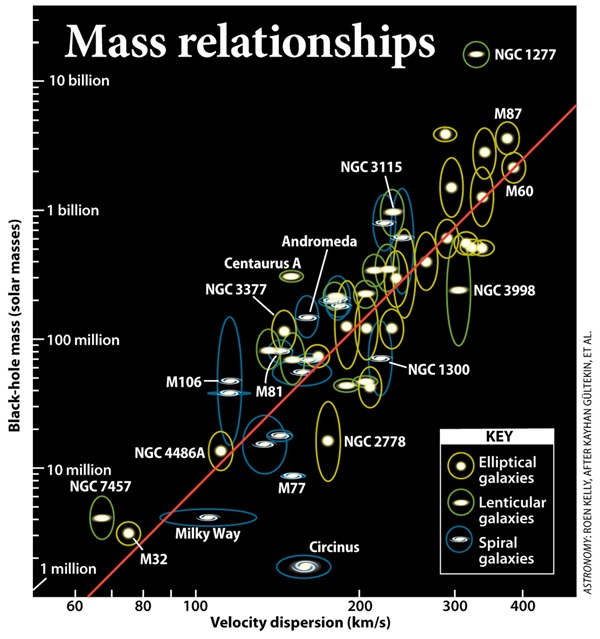
What to notice: central black-hole mass increases with the random motions of stars in the galaxy bulge. The plot is not saying the black hole directly controls the whole bulge; it is showing that the black hole and bulge somehow grew in linked ways. (Credit: Astronomy: Roen Kelly, after Kayhan Gultekin et al.)
The plot connects two different kinds of inference:
- black-hole mass, inferred from motions of stars or gas near the center,
- bulge velocity dispersion, inferred from Doppler-broadened stellar absorption lines.
This is not a direct movie of black holes and galaxies growing together. It is an evidence pattern built from measurements of light and motion.
This correlation is surprising because the black hole is tiny compared with the galaxy. Even a billion-solar-mass black hole directly dominates gravity only in the central region. The galaxy bulge extends across thousands of light-years.
One leading explanation is AGN feedback. When the black hole accretes gas, radiation, winds, and jets can heat or expel gas from the galaxy. That can reduce both star formation and further black-hole feeding.
But the correlation alone does not prove the mechanism. It tells us that black-hole growth and galaxy growth are linked. Explaining the link requires a physical model.
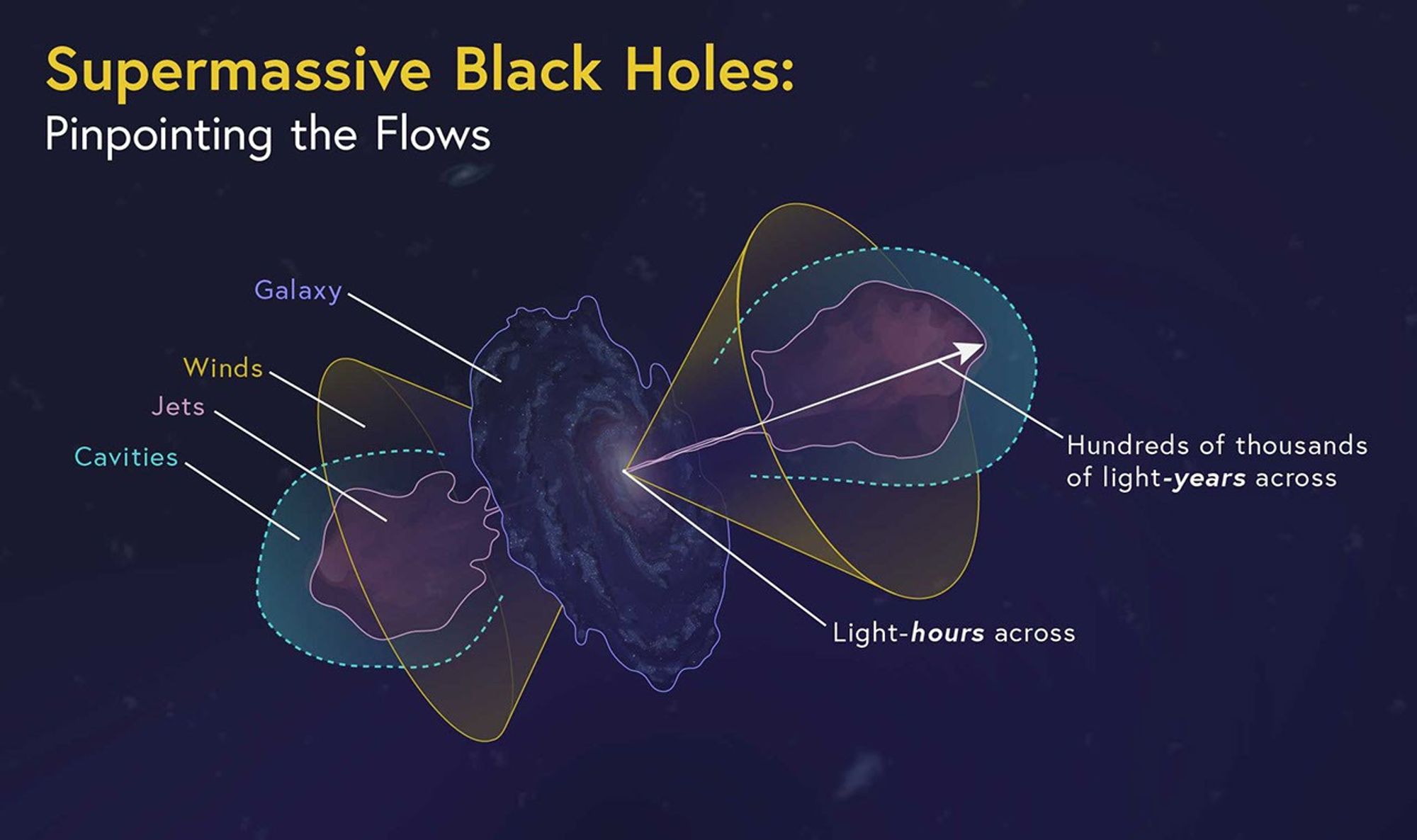
What to notice: AGN energy does not stay near the event horizon. Jets, winds, and cavities connect light-hour scales near the black hole to galaxy-scale environments. (Credit: NASA)
AGN feedback is a galaxy-scale claim about energy flow. Jets, winds, and cavities are evidence that the central engine can affect gas far beyond the immediate black-hole environment.
The \(M\)-\(\sigma\) relation connects black-hole mass to the velocity dispersion of bulge stars.
Before reading the answer, identify:
- What do astronomers directly observe?
- What requires a model?
- Why does that distinction matter?
Astronomers directly observe light.
For the bulge, they observe broadened stellar absorption lines. The broadening tells us that stars in the bulge have a range of line-of-sight velocities.
The velocity dispersion \(\sigma\) is inferred from those spectra. The bulge mass and black-hole mass require dynamical models that connect motion to gravity.
This distinction matters because the \(M\)-\(\sigma\) relation is not based on directly seeing a black hole “control” a galaxy. It is based on translating light into velocities, and velocities into gravitational mass.
The Cosmic Web
Now zoom out again.
Galaxies are not scattered randomly through space. They collect into:
- groups, like the Local Group,
- clusters, containing hundreds to thousands of galaxies,
- filaments, long chains of galaxies and gas,
- walls, broad sheet-like structures,
- voids, large regions with relatively few galaxies.
Together, this pattern is called the cosmic web.
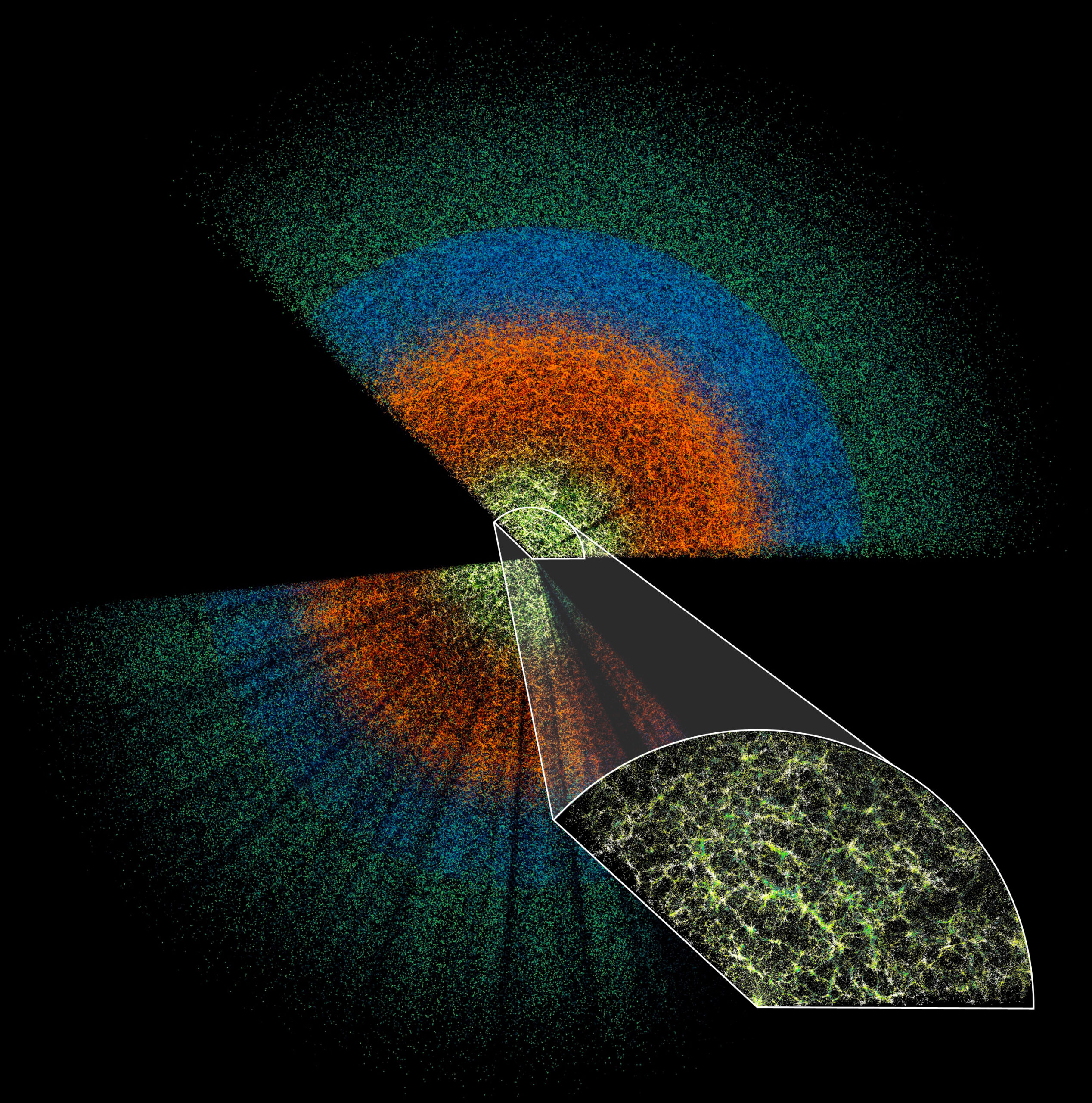
What to notice: every point is a galaxy with a measured redshift. The cosmic web is not a drawing; it is the pattern that appears when distances are added to sky positions. (Credit: NSF NOIRLab/DESI Collaboration)
A cosmic-web map is not just a sky image. Each point is a galaxy with a measured position and distance. The web appears only when astronomers add distance information to sky position.
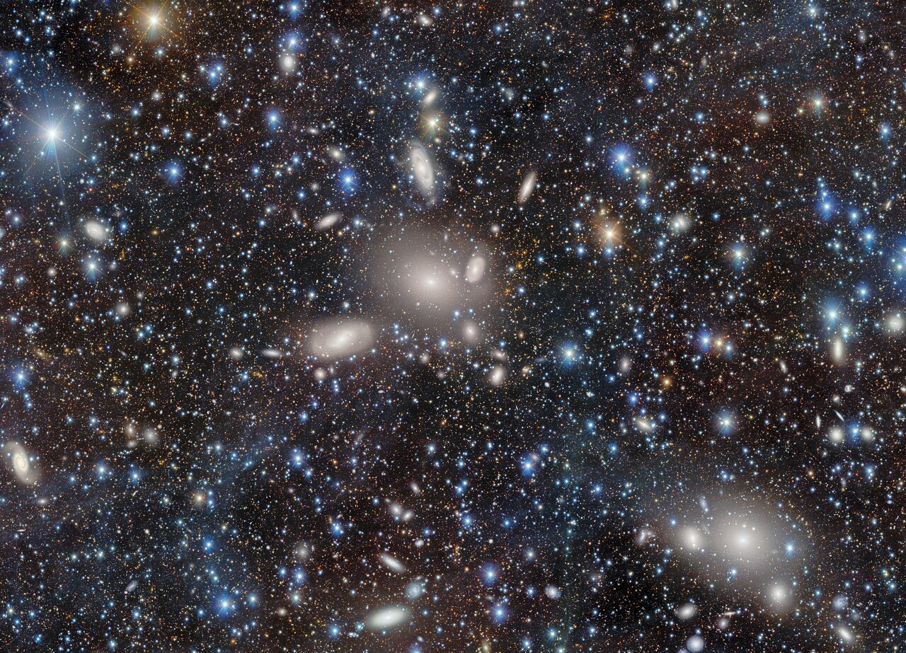
What to notice: a galaxy cluster is not a single object but a gravitational city of galaxies. The Antlia Cluster lets students see the step from individual galaxies to environments where galaxies live together. (Credit: NSF NOIRLab)
A cluster is a dense node in the web. Many galaxies occupy the same gravitational environment, so the cluster is evidence for a large concentration of underlying mass.
The physical model is gravitational growth.
In the early universe, matter was almost uniform, but not perfectly uniform. Some regions were slightly denser than average. Gravity amplified those small differences over time.
- Dense regions pulled in more matter and became clusters.
- Connecting regions became filaments.
- Underdense regions emptied out and became voids.
Dark matter is essential here. Most of the matter shaping the cosmic web is not in stars. Galaxies are bright tracers of a larger dark-matter structure.
Observable: Galaxies form filaments, clusters, walls, and voids.
Model: Gravity amplifies small early density differences, with dark matter providing most of the mass.
Inference: The cosmic web is the large-scale structure of matter in the universe, traced by galaxies.
Galaxies show us where the web is, but they are not most of the mass. The web is primarily a dark-matter structure, with galaxies acting as visible tracers.
Distance Ladder Check-In
This lecture introduced the distance problem. The rest of Module 3 builds the solution.
| Rung | Method | What it measures | Approximate reach |
|---|---|---|---|
| 1 | Radar ranging | Solar System distances | AU scale |
| 2 | Stellar parallax | Nearby stellar distances | kpc scale for useful cases |
| 3 | Main-sequence fitting | Star-cluster distances | Milky Way and nearby satellites |
| 4 | Cepheid variables | Distances to nearby galaxies | tens of Mpc |
| 5 | Type Ia supernovae | Distances to far galaxies | thousands of Mpc |
| 6 | Hubble’s law | Cosmological expansion distances | largest scales |
The distance ladder works because each rung calibrates the next.
Nearby geometry calibrates stars.
Stars calibrate galaxies.
Galaxies reveal cosmic expansion.
Lectures 24-26 will use this ladder to connect galaxy distances to Hubble’s law, dark energy, and the early universe.
Deep Dives (Optional)
AGN come with a confusing zoo of historical names: Seyferts (Type 1 and 2), radio galaxies, quasars, BL Lacs, blazars. The Unified Model proposes that most of these differences come from viewing angle: the same basic object (SMBH + accretion disk + torus + jets) looks different depending on whether you see it face-on (quasar, blazar), edge-on through the torus (Type 2 Seyfert), or somewhere in between (Type 1 Seyfert). Some differences are real (e.g., radio-loud vs. radio-quiet AGN differ in jet power), but orientation does much of the zoological work.
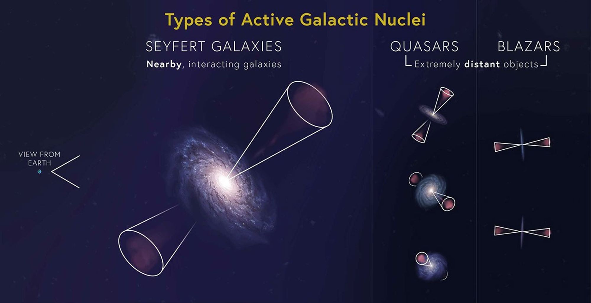
What to notice: many AGN names partly encode viewing angle. The same basic engine can look like a Seyfert galaxy, quasar, or blazar depending on how the disk, torus, and jets point toward us. (Credit: NASA)
The unified model connects names to viewing angle. The same central engine can look different depending on whether the disk, torus, and jet point toward us.
Cepheid variables are pulsating giants whose pulsation period is set by their mean density, which is in turn set by their luminosity. More luminous Cepheids pulsate more slowly. This is why \(L\) can be read off from the period \(P\), an extraordinary fact that was discovered empirically by Henrietta Leavitt in 1912 and later understood theoretically as a consequence of stellar structure. Lecture 24 develops this argument in detail.
Misconceptions
The Hubble sequence is a classification system, not an evolutionary timeline. Galaxies can change type through mergers, gas loss, gas accretion, and star-formation shutdown, but they do not simply move along the tuning fork in order.
Apparent brightness depends on both luminosity and distance. A faraway quasar can look bright because it is intrinsically enormous in luminosity. A nearby dwarf galaxy can look faint because it is intrinsically dim.
A quasar is not powered by fusion. It is powered by accretion onto a supermassive black hole in the center of a galaxy.
Visible light is only one window. Radio, infrared, ultraviolet, and X-ray observations reveal gas, dust, star formation, jets, hot plasma, and black-hole activity that visible light alone can miss.
Galaxies trace the cosmic web, but most of the matter shaping the web is dark matter. The galaxies are the visible markers of a larger gravitational structure.
Practice Problems
Solutions are available in the Lecture 23 Solutions.
Core Problems (Start Here)
Problem 1: Classify It
You are handed four galaxy images.
- Galaxy X is a smooth red ellipsoid with no visible dust lanes or H II regions.
- Galaxy Y has tightly wound spiral arms, a large central bulge, and some pink H II regions along the arms.
- Galaxy Z has no clear symmetry, is blue, and is full of bright knots of young stars.
- Galaxy W has a straight bright bar through its center, with spiral arms beginning near the ends of the bar and many pink H II regions along the arms.
Classify each galaxy as elliptical, spiral, barred spiral, or irregular. Then rank, or group, the galaxies from most to least ongoing star formation based on the evidence given.
Problem 2: Why Parallax Is Not Enough
Andromeda is about \(780\ {\rm kpc}\) away. Ordinary stellar parallax becomes extremely difficult at such distances.
In two or three sentences, explain why Cepheid variables are useful for measuring Andromeda’s distance.
Your answer should mention:
- what we observe,
- what we infer,
- why a standard candle helps.
Problem 3: Quasar Luminosity
A quasar has observed flux:
\[ F = 10^{-14}\ {\rm W\,m^{-2}} \]
Its distance is:
\[ d = 3\ {\rm Gpc} \approx 9 \times 10^{25}\ {\rm m} \]
Use:
\[ L = 4\pi d^2 F \]
to estimate its luminosity.
Then compare your answer to the Sun’s luminosity:
\[ L_\odot = 3.8 \times 10^{26}\ {\rm W} \]
How many Suns is the quasar equivalent to?
Problem 4: Eddington Mass Lower Bound
Use your answer from Problem 3. It should be close to:
\[ L \sim 10^{39}\ {\rm W} \]
The Eddington luminosity is approximately:
\[ L_{\rm Edd} \approx 1.3 \times 10^{31}\ {\rm W}\left(\frac{M}{M_\odot}\right) \]
Estimate the minimum black-hole mass needed to power this quasar if it is radiating near the Eddington limit.
Problem 5: Reading a Cosmic-Web Map
Return to the DESI redshift-survey map in the Cosmic Web section above, or use an equivalent SDSS/DESI galaxy survey map.
Identify:
- a cluster,
- a filament,
- a void.
For each one, write one sentence explaining what you infer about the underlying dark-matter distribution.
Challenge Problems (Deepen Your Understanding)
Challenge 1: Fusion vs. Accretion Efficiency
Hydrogen fusion converts about \(0.7\%\) of mass energy into radiation. Black-hole accretion can convert several percent to tens of percent.
In one paragraph, explain why this efficiency difference matters for quasars.
Your answer should address:
- why quasars need an extremely efficient power source,
- why ordinary stars cannot explain rapid quasar variability,
- why accretion onto a supermassive black hole is a better model.
Challenge 2: Reading the \(M\)-\(\sigma\) Relation
Suppose the approximate trend is:
\[ M_{\rm SMBH} \propto \sigma^4 \]
Galaxy A has:
\[ \sigma_A = 100\ {\rm km\,s^{-1}} \]
Galaxy B has:
\[ \sigma_B = 200\ {\rm km\,s^{-1}} \]
By what factor would you expect Galaxy B’s black hole mass to exceed Galaxy A’s?
Then explain why this kind of relation is evidence for linked galaxy and black-hole growth, but not by itself proof of AGN feedback.
Challenge 3: Feedback as a Thermostat
Write one paragraph explaining the idea of AGN feedback as a thermostat.
Use this structure:
- If the black hole accretes rapidly, then…
- This affects the surrounding gas by…
- That changes star formation because…
- Therefore black-hole growth and galaxy growth may become linked because…
Reading Summary
Galaxies are not just distant smudges. Their shapes, colors, spectra, gas content, and environments are evidence.
Galaxy morphology sorts galaxies into ellipticals, spirals, barred spirals, and irregulars. These categories are clues about stellar populations, gas content, star formation, and interaction history.
Distance is the central measurement problem. Without distance, apparent brightness and apparent size cannot be converted into luminosity and physical size.
Standard candles solve the distance problem. If we know an object’s luminosity \(L\) and measure its flux \(F\), we can infer distance using the inverse-square law.
Quasars and AGN are powered by accretion, not fusion. Gas falling toward a supermassive black hole can release energy far more efficiently than ordinary stellar fusion.
The Eddington limit links luminosity to black-hole mass. Extremely luminous quasars require very massive black holes.
The \(M\)-\(\sigma\) relation suggests co-evolution. Black-hole mass is correlated with the motions of stars in the host galaxy’s bulge, implying that galaxy growth and black-hole growth are connected.
The cosmic web is the large-scale structure of matter. Galaxies trace filaments, clusters, walls, and voids shaped primarily by dark matter and gravity.
The main skill from this lecture is not memorizing galaxy names. It is learning how astronomers turn images and spectra into physical histories.
Glossary
Accretion: The process of gas falling onto a compact object, such as a black hole. In an accretion disk, gravitational energy is converted into heat and light.
Active galactic nucleus (AGN): A bright central region of a galaxy powered by gas accreting onto a supermassive black hole.
Barred spiral: A spiral galaxy with a straight bar-shaped structure through its center.
Cosmic web: The large-scale pattern of galaxies, gas, and dark matter arranged into filaments, clusters, walls, and voids.
Dark matter: Matter that does not emit or absorb light but has gravity. It shapes galaxy rotation, galaxy clusters, and the cosmic web.
Elliptical galaxy: A smooth, rounded or elongated galaxy usually dominated by older stars and relatively little cold gas.
Flux: The amount of energy received per second per square meter at a detector. Flux depends on both luminosity and distance.
H II region: A cloud of ionized hydrogen around young, hot stars. H II regions are evidence of recent star formation.
Hubble sequence: A galaxy classification system based on visual morphology, including ellipticals, spirals, barred spirals, and irregulars.
Irregular galaxy: A galaxy without a clear spiral or elliptical structure, often gas-rich and actively forming stars.
Luminosity: The total power emitted by an object. Luminosity is intrinsic; it does not depend on distance.
Quasar: An extremely luminous AGN powered by accretion onto a supermassive black hole.
Spiral galaxy: A disk galaxy with spiral arms, gas, dust, and ongoing star formation.
Standard candle: An object whose luminosity can be estimated from its physics, allowing astronomers to infer distance from observed flux.
Supermassive black hole: A black hole with a mass of millions to billions of solar masses, usually found in the centers of galaxies.
Velocity dispersion: A measure of how widely stellar speeds vary in a system such as a galaxy bulge.
Looking Ahead
Next lecture (Lecture 24) is where we close the distance-ladder gap that this reading opened. We will walk through Cepheid variables in detail (Henrietta Leavitt’s period-luminosity relation), connect them to the Type Ia supernovae that will appear in Lecture 25, and use them to derive Hubble’s law, the relation between a galaxy’s distance and its recession velocity that is the observational foundation of modern cosmology. We will also meet the Hubble tension, one of the most interesting open problems in modern astrophysics.
After that, Type Ia supernovae give us the accelerating universe and dark energy (Lecture 25), and the cosmic microwave background takes us all the way back to 380,000 years after the Big Bang (Lecture 26).
Dark matter is the first of three hidden things (Lecture 22, and already showing up in the cosmic web here). Dark energy is the second (Lecture 25). The origin of the elements, including the ones in your body, is the third (Lecture 26). Every one of them depends on stars.