Lecture 24: The Distance Ladder and Hubble’s Law
How We Measure the Universe, and Why It’s Expanding
The Big Idea
On sufficiently large scales, galaxy redshifts obey a simple rule: the farther a galaxy is, the faster it recedes from us. Nearby galaxies can have their own local motions — Andromeda is the famous blueshifted exception — but once cosmic expansion dominates over local gravity, the pattern is unmistakable. That rule, Hubble’s law, is not a statement about motion through space; it is a statement about the expansion of space itself. Combined with a cosmic distance ladder built rung by rung from parallax to Cepheid variables to Type Ia supernovae, Hubble’s law gives us an age and size for the observable universe. And the fact that two different ways of measuring \(H_0\) disagree tells us we may not understand the expansion as well as we thought.
Observable: Galaxies have redshifted spectral lines, and standard candles give distances to some of those galaxies.
Model: The distance ladder calibrates luminosities, while expanding-space cosmology connects redshift, distance, and expansion rate.
Inference: The universe is expanding, and the present-day expansion rate \(H_0\) sets a rough age and distance scale for the observable universe.
Main uncertainty: The local ladder depends on calibrated astrophysical rungs; the CMB value depends on fitting an early-universe model. The Hubble tension asks whether one side has hidden systematics or whether the model is incomplete.
This page answers four questions:
- How do we measure distances to galaxies?
- What is the relation between a galaxy’s distance and its redshift?
- What does that relation tell us about the age and size of the universe?
- Why do two different measurements of the expansion rate disagree — and what could that mean?
Punchline: Standard candles tell us how far. Redshifts tell us how fast. Together they give us \(H_0\), the age of the universe, and the observable horizon. Stars are the rung we climb on.
This reading is the most important quantitative section of Module 3. If you understand the distance ladder and Hubble’s law, the rest of cosmology (Lectures 25 and 26) is a refinement on this foundation.
Default expectation (best): Read the whole page before lecture. Work all the Check Yourself problems with pencil and paper.
If you’re short on time (~25 min): Focus on:
- The Big Idea above
- The Distance Ladder section (all five rungs)
- Cepheid Variables and the Leavitt Relation
- Hubble’s Law
- The Hubble Tension
Goal after 25 minutes: You should be able to (a) name each rung of the distance ladder and what it calibrates, (b) state Hubble’s law, and (c) explain why it says the universe is expanding, not that galaxies are flying through space.
Reference mode: The Distance Ladder Reference Box and the \(H_0\) table are the long-term study references.

What to notice: Module 3 uses the same evidence chain over and over. Dust, 21-cm emission, S-star orbits, galaxy shapes, Cepheid periods, supernova brightness, redshifts, AGN jets, CMB anisotropies, and light-element abundances become physical claims only after a model translates them. (Credit: Illustration: A. Rosen (SVG))
Learning Outcomes
By the end of this reading, you should be able to say:
The Problem That Will Not Go Away
Every galaxy in the sky is some distance from us. That distance is what converts what we measure (apparent flux, apparent size, apparent angular extent) into what we want to know (luminosity, physical size, physical mass). Without a distance, we are looking at a projection — a two-dimensional sky with a third dimension hidden behind it.
Lecture 23 introduced standard candles — objects of known luminosity \(L\) whose apparent brightness \(F\) lets us solve for distance via
\[ d = \sqrt{\frac{L}{4\pi F}} \]
But what makes an object “standard”? And how do we calibrate its \(L\) in the first place? The answer is that we do not do it all at once. We build a distance ladder, where each rung is calibrated by the one below it.
The Cosmic Distance Ladder
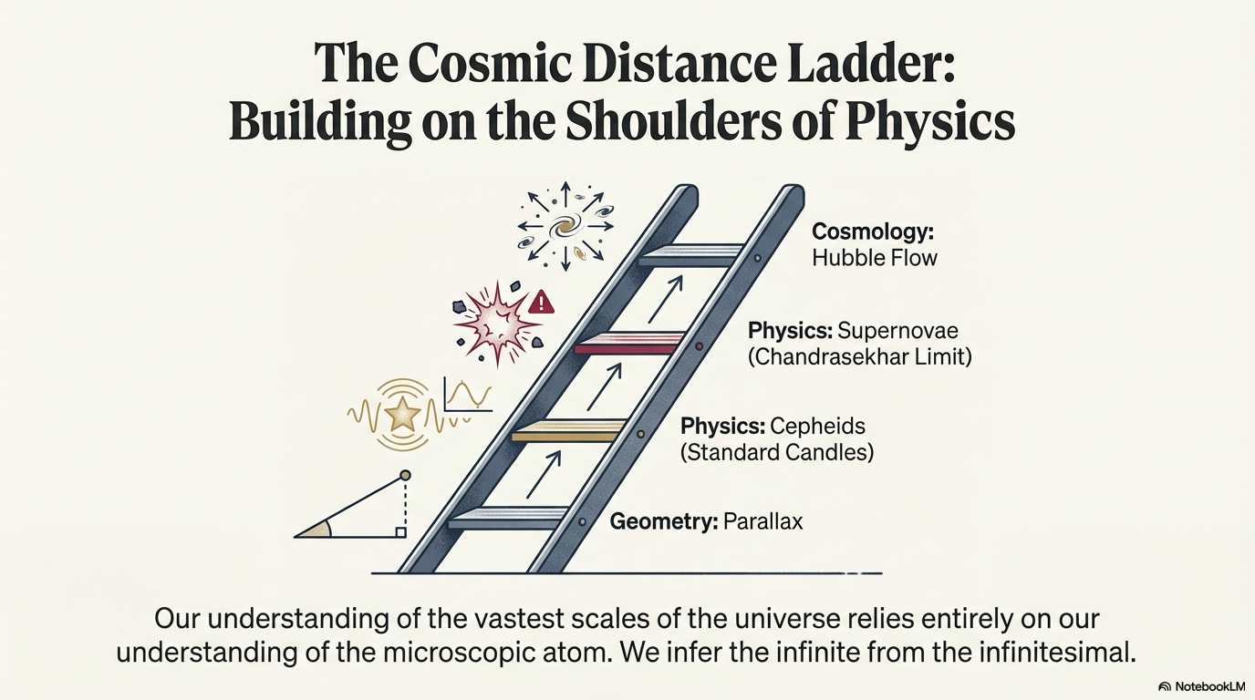
What to notice: Each rung calibrates the next. Parallax (geometry) → Cepheids (standard candles) → Supernovae (Chandrasekhar limit) → Hubble Flow (cosmology). We infer the infinite from the infinitesimal. (Credit: (A. Rosen/NotebookLM))
Rung 1 — Radar Ranging (Solar System)
Inside the Solar System, we measure distances directly by bouncing radar off planets. We know the time light takes to travel out and back, and we know \(c\), so \(d = c \, t / 2\). This fixes the astronomical unit (AU) to very high precision: \(1\ {\rm AU} = 1.496 \times 10^{11}\ {\rm m}\). This rung is essentially exact and anchors everything above it.
Rung 2 — Stellar Parallax
For stars within about \(1\ {\rm kpc}\), we use parallax: the apparent shift of a nearby star against more distant background stars as Earth orbits the Sun. A star at distance \(d\) in parsecs has a parallax angle of
\[ p\ {\rm (arcsec)} = \frac{1}{d\ {\rm (pc)}} \]
Gaia’s astrometric mission has measured parallaxes for nearly a billion stars, reaching usefully to distances of about \(3\) to \(5\ {\rm kpc}\) for the brightest stars but about \(1\ {\rm kpc}\) for reliable precision on most individual stars.

What to notice: Gaia does not merely improve one nearby distance here or there. Its parallax reach extends across a large fraction of the Milky Way, turning local geometry into a three-dimensional galactic map.
Parallax is the first truly distance-calibrated rung. It depends only on geometry and the size of Earth’s orbit (Rung 1).
Rung 3 — Spectroscopic Parallax and Main-Sequence Fitting
Beyond Gaia parallax, we use the H-R diagram itself (Lecture 16). If we know a star’s spectral type (from its spectrum) and can locate it on the H-R diagram, we know its absolute luminosity \(L\) to within about a factor of \(2\). Apparent brightness then gives distance.
For star clusters, this idea sharpens: a cluster’s main sequence has a fixed shape (calibrated from nearby clusters via parallax), and its apparent main sequence is shifted vertically by the cluster’s distance modulus. This is called main-sequence fitting and reaches about \(100\ {\rm kpc}\).
Rung 4 — Cepheid Variables
Here is where stars begin to do the real cosmological work. The discovery of the Cepheid period-luminosity relation is a short story worth knowing.
In 1912, Henrietta Leavitt — a “computer” at Harvard College Observatory — noticed that a class of pulsating stars in the Small Magellanic Cloud (SMC) had a remarkable property: their period of brightness variation was tightly correlated with their mean brightness. Because every star in the SMC is at essentially the same distance from us, differences in apparent brightness were differences in intrinsic luminosity. Leavitt had found a relation between period and luminosity:
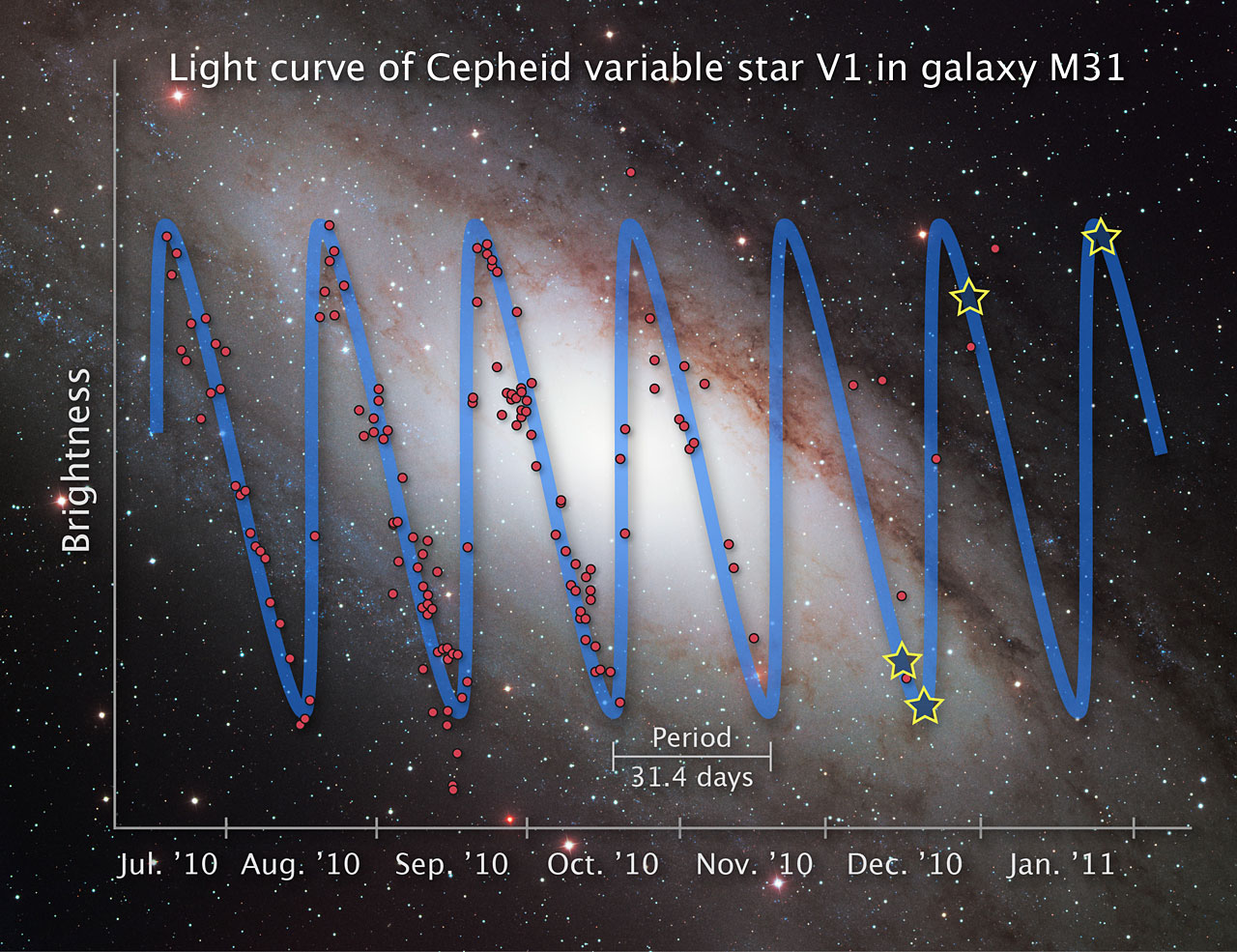
What to notice: a Cepheid’s period is directly observable. Repeated brightness measurements turn a distant unresolved star into a clock, and that clock predicts the star’s luminosity. (Credit: ESO)
\[ \log_{10} L = a \log_{10} P + b \]
with \(P\) measured in days. Longer-period Cepheids are intrinsically more luminous. Modern calibrations give (approximately):
\[ L \approx 335\,L_\odot \left( \frac{P}{1\ {\rm day}} \right)^{1.15} \]
for classical Cepheids. A \(10\)-day Cepheid is about \(4{,}700\ L_\odot\). A \(100\)-day Cepheid is about \(65{,}000\ L_\odot\).
The numerical coefficients in the Leavitt relation (here 335 and 1.15) depend on wavelength band, zero-point calibration, and metallicity corrections. Modern calibrations in the literature (Madore & Freedman; Riess et al.; the Hubble Space Telescope Key Project) agree within a few tens of percent but are not identical. The relation we use here is a representative bolometric form suitable for order-of-magnitude distance estimates. For actual distance-ladder work, astronomers use carefully calibrated near-infrared relations with explicit metallicity corrections.
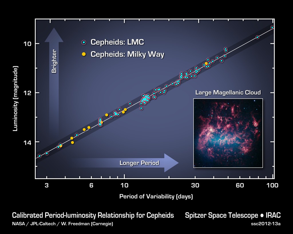
What to notice: longer-period Cepheids are intrinsically brighter. This plot is the ladder step: period is easy to measure, luminosity follows from the relation, and flux then gives distance. (Credit: NASA/IPAC Extragalactic Database)
This is the key move: the period, which we can measure from a distant galaxy, tells us the luminosity, which lets us compute distance. The calibration comes from nearby Cepheids whose distances we know from parallax (Rung 2) or cluster fitting (Rung 3).
Cepheids are bright (supergiants, \(10^3\) to \(10^5\,L_\odot\)), so they are visible out to about \(30\ {\rm Mpc}\) with Hubble Space Telescope. This is far enough to reach the Virgo Cluster (about \(16\ {\rm Mpc}\)) and dozens of nearby galaxies, including ones that have hosted Type Ia supernovae.
Cepheids are specific kinds of stars in a specific evolutionary phase — giants on an instability strip where their envelopes pulsate due to ionization-recombination of helium. The very physics of the pulsation (you can think of it as helium acting as a valve) sets the period-luminosity relation. Without stellar physics, we would have no cosmic distance ladder beyond parallax.
You observe a Cepheid in a nearby galaxy. Its pulsation period is \(30\ {\rm days}\) and its apparent flux is \(F = 10^{-14}\ {\rm W\,m^{-2}}\). Estimate:
- The Cepheid’s luminosity \(L\) in solar units.
- The distance \(d\) to the host galaxy in Mpc (\(1\ {\rm Mpc} = 3.09 \times 10^{22}\ {\rm m}\)).
- Using \(L \approx 335\,L_\odot (P/{\rm day})^{1.15}\) with \(P = 30\):
\[ L \approx 335 \times 30^{1.15}\,L_\odot \approx 335 \times 49\,L_\odot \approx 1.6 \times 10^4\,L_\odot \]
Convert:
\[ L \approx 1.6 \times 10^4 \times 3.8 \times 10^{26}\ {\rm W} \approx 6 \times 10^{30}\ {\rm W} \]
- From \(d = \sqrt{L / (4\pi F)}\):
\[ d = \sqrt{\frac{6 \times 10^{30}}{4\pi \times 10^{-14}}}\ {\rm m} \approx \sqrt{4.8 \times 10^{43}}\ {\rm m} \approx 7 \times 10^{21}\ {\rm m} \]
In Mpc:
\[ d \approx \frac{7 \times 10^{21}}{3.09 \times 10^{22}} \approx 0.2\ {\rm Mpc} \]
This is about \(230\ {\rm kpc}\), beyond the Large and Small Magellanic Clouds and at roughly the distance scale of the Local Group’s outer dwarf galaxies. For reference: a Cepheid of this same luminosity at the SMC distance, about \(60\ {\rm kpc}\), would produce \(F \sim 1.5 \times 10^{-13}\ {\rm W\,m^{-2}}\), about \(15\times\) brighter than the flux given in this problem.
Rung 5 — Type Ia Supernovae (Preview)
Cepheids peter out at about \(30\ {\rm Mpc}\). To go farther we need something brighter. Type Ia supernovae are our tool. They reach peak luminosities of \(\sim 5 \times 10^9\,L_\odot\) — comparable to an entire small galaxy — and can be seen out to thousands of Mpc.
Crucially, they are approximately standard: they all explode from (roughly) the same physical configuration, so their peak luminosities fall in a narrow range that can be further tightened using the shape of their light curve (the Phillips relation).
Type Ia SNe are calibrated on Cepheids — we measure Cepheids in nearby galaxies that have also hosted Type Ia SNe, which fixes the Type Ia peak luminosity. That calibrated Type Ia luminosity is then applied to very distant SNe to measure cosmic distances.
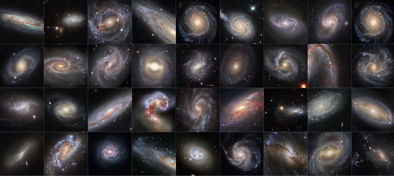
What to notice: Type Ia supernova calibration is a host-galaxy problem. Cepheids in nearby galaxies set the distance to the host, and that distance calibrates any Type Ia supernova that appeared there. (Credit: NASA/ESA/Hubble)
Lecture 25 gives the full stellar-physics story — what explodes, why, and why the peak luminosity is (nearly) universal. For now, we use them as “ultra-bright Cepheids.”
Rung 6 — Hubble’s Law
Once we have distances out to a few hundred Mpc, a new relation becomes usable. It is the subject of the rest of this reading.
| Rung | Method | Reach | Calibrator |
|---|---|---|---|
| 1 | Radar ranging | ~AU | Physical constants |
| 2 | Parallax | about \(1\) to \(5\ {\rm kpc}\) | Rung 1 (Earth orbit) |
| 3 | Spectroscopic parallax / main-sequence fitting | about \(100\ {\rm kpc}\) | Rung 2 |
| 4 | Cepheid variables | about \(30\ {\rm Mpc}\) | Rungs 2 to 3 |
| 5 | Type Ia supernovae | about \(10^3\ {\rm Mpc}\) | Rung 4 |
| 6 | Hubble’s law (redshift \(\to\) distance) | cosmological | Rungs 4 to 5 |
Each rung calibrates the rung above it. Break any rung and the upper ones wobble.
Suppose a Type Ia supernova goes off in a galaxy that also contains Cepheid variables. Which object gives the distance to the galaxy directly, and which object gets calibrated so it can be used much farther away?
The Cepheids give the distance to the nearby host galaxy because their period-luminosity relation has already been calibrated by lower rungs such as parallax. The Type Ia supernova is then calibrated: once we know its host distance, we can infer its corrected peak luminosity and use similar Type Ias in much more distant galaxies.
Hubble’s Law
Hubble’s Discovery
In 1929, Edwin Hubble published a plot of galaxy recession velocities (measured from Doppler-shifted absorption lines) against distances (estimated from Cepheids in those galaxies). The result: a roughly linear relation. Farther galaxies recede faster.
What to notice: Hubble’s law is a slope. Redshift gives recession velocity, independent distance measurements set the horizontal axis, and the best-fit line gives \(H_0\). (Credit: Course-provided figure)
The relation is written
\[v = H_0 \, d\]
where:
- \(v\) is the galaxy’s recession velocity (inferred from its redshift),
- \(d\) is the distance,
- \(H_0\) is the Hubble constant, the slope of the line.
Representative recent values of \(H_0\) cluster around \(67\) to \(73\ {\rm km\,s^{-1}\,Mpc^{-1}}\), depending on the method. A galaxy \(100\ {\rm Mpc}\) away recedes at roughly \(7{,}000\ {\rm km\,s^{-1}}\). A galaxy \(1\ {\rm Gpc}\) away recedes at roughly \(70{,}000\ {\rm km\,s^{-1}}\), about a quarter of the speed of light.
What Hubble’s Law Is Not
Hubble’s law is not a statement that galaxies are flying outward through space from some special center. If it were, we would be at the center of a cosmic explosion, which is implausible — and worse, galaxies in every direction recede. Instead:
Hubble’s law says space itself is expanding.
Imagine dots painted on the surface of a balloon. As the balloon inflates, every dot sees every other dot move away, and more-distant dots move away faster. No dot is at the center. Space is doing the expanding; the dots are carried along.
Imagine three galaxies painted on an expanding balloon: A and B are close together, while A and C are twice as far apart.
If the balloon doubles in size, which separation grows by the larger amount: A-B or A-C? Which pair has the larger recession speed?
Use this to explain why Hubble’s law is a slope: more distance means more expanding space between galaxies.
The redshift is not really a Doppler shift (though for small distances the math is the same). It is a cosmological redshift — light stretched by the expansion of space during its travel from source to us.
What to notice: redshift is measured by matching spectral fingerprints. The same absorption-line pattern appears at longer wavelengths in the observed spectrum, so the shift is a measurement, not a color impression. (Credit: NASA)
The observable is the pattern of spectral lines. If the whole fingerprint appears shifted to longer wavelengths, we infer that space expanded while the light was traveling.
What to notice: expanding space stretches traveling light. Bound objects such as galaxies keep their size, while the space between galaxies grows and increases the wavelength of light in transit. (Credit: NASA)
This NASA SVS animation shows the key physical idea behind cosmological redshift: as the universe expands, the wavelength of traveling light stretches along with space. Watch for the evidence-chain distinction: the animation is a model picture, while the observable is the shift of known spectral features to longer wavelengths.
A galaxy has a measured recession velocity of \(v = 15{,}000\ {\rm km\,s^{-1}}\). Use \(H_0 = 70\ {\rm km\,s^{-1}\,Mpc^{-1}}\) to estimate its distance.
\[ d = \frac{v}{H_0} = \frac{15{,}000}{70}\ {\rm Mpc} \approx 214\ {\rm Mpc} \]
This is roughly the distance at which Type Ia supernovae become essential, because Cepheids alone cannot reach this far. It is also well within the Hubble flow regime where peculiar velocities from local gravitational effects are small compared to the Hubble velocity.
The Hubble Time and Age of the Universe
If the universe has been expanding at a constant rate, then the time since it was all at one point is
\[ t_H = \frac{1}{H_0} \]
This is called the Hubble time. Let’s convert units for \(H_0 = 70\ {\rm km\,s^{-1}\,Mpc^{-1}}\):
\[ H_0 = 70 \frac{{\rm km\,s^{-1}}}{{\rm Mpc}} = 70 \frac{{\rm km\,s^{-1}}}{3.09 \times 10^{19}\ {\rm km}} = 2.27 \times 10^{-18}\ {\rm s^{-1}} \]
So \(t_H = 1 / H_0 \approx 4.4 \times 10^{17}\) s \(\approx 14\) Gyr.
This is a rough estimate. The actual age of the universe — 13.8 Gyr — differs from \(t_H\) by a small factor that depends on whether the expansion has been speeding up or slowing down (Lecture 25). But the order of magnitude is right.
Repeat the calculation with \(H_0 = 67\ {\rm km\,s^{-1}\,Mpc^{-1}}\) (the CMB-based value; Lecture 26) and \(H_0 = 73\ {\rm km\,s^{-1}\,Mpc^{-1}}\) (the Cepheid-SNIa local value). What are the two estimates of \(t_H\)?
\(H_0 = 67\ {\rm km\,s^{-1}\,Mpc^{-1}} = 2.17 \times 10^{-18}\ {\rm s^{-1}}\), so \(t_H \approx 4.6 \times 10^{17}\ {\rm s} \approx 14.6\ {\rm Gyr}\).
\(H_0 = 73\ {\rm km\,s^{-1}\,Mpc^{-1}} = 2.37 \times 10^{-18}\ {\rm s^{-1}}\), so \(t_H \approx 4.2 \times 10^{17}\ {\rm s} \approx 13.4\ {\rm Gyr}\).
Both are within ~1 Gyr of the best-fit age (13.8 Gyr), and the two values differ from each other by about 1.2 Gyr — which brings us to the Hubble tension.
Worked Example: From Redshift to a Distance
Given: A galaxy’s spectrum shows a hydrogen line at \(\lambda_{\text{obs}} = 670\ {\rm nm}\). Its laboratory (rest-frame) wavelength is \(\lambda_0 = 656.3\ {\rm nm}\) (H\(\alpha\)). Use \(H_0 = 70\ {\rm km\,s^{-1}\,Mpc^{-1}}\).
Relation: For \(v \ll c\), the cosmological redshift reduces to a Doppler-like form: \[ z = \frac{\lambda_{\text{obs}} - \lambda_0}{\lambda_0}, \qquad v \approx c\,z, \qquad d = \frac{v}{H_0} \]
Rearrange for distance directly in terms of redshift: \[ d = \frac{c\,z}{H_0} \]
Substitute: \[ z = \frac{670 - 656.3}{656.3} = 0.0209, \qquad v \approx (3 \times 10^5\ {\rm km\,s^{-1}}) \times 0.0209 \approx 6{,}270\ {\rm km\,s^{-1}} \]
Evaluate: \[ d = \frac{6{,}270}{70}\ {\rm Mpc} \approx 90\ {\rm Mpc} \]
Interpret: The galaxy is about \(90\ {\rm Mpc}\) away — well beyond the reach of Cepheids alone and deep in the Hubble flow, so its peculiar velocity is a small correction. Notice that the entire calibration of this answer traces back through Type Ia SNe \(\to\) Cepheids \(\to\) parallax: without stars, the Hubble constant we just used would have no numerical value at all. This calculation is the low-redshift limit; for \(z \gtrsim 0.1\), relativistic corrections and the time-dependence of \(H\) make \(d(z)\) more complicated.
The Observable Universe
Because the universe has a finite age, there is a finite distance from which light has had time to reach us. This is the observable horizon. Its rough scale is the Hubble distance:
\[ d_H = \frac{c}{H_0} \approx 4.3\ {\rm Gpc} \]
for \(H_0 = 70\ {\rm km\,s^{-1}\,Mpc^{-1}}\). This is about \(14\) billion light-years.
Do not confuse three related scales:
- Hubble distance: about \(14\ {\rm Gly}\), from \(c/H_0\).
- Observable-universe comoving radius: about \(46\ {\rm Gly}\), because space expanded while the light traveled.
- Observable-universe comoving diameter: about \(92\ {\rm Gly}\).
The Hubble distance is therefore a scale marker, not the radius of everything we can observe.
Use the wavelength buttons to compare infrared, visible, ultraviolet, X-ray, and multiwavelength views of the same deep field. This is the observational version of the phrase “lookback time”: distant galaxies are not just far away; their light left when the universe was younger.
What to notice: each wavelength selects a different physical process. Infrared highlights dust and old/redshifted starlight, ultraviolet highlights star formation, X-rays reveal actively growing black holes, and the composite turns one patch of sky into a timeline of galaxy evolution.
The Hubble Tension
Here is the current problem. We have two independent ways to measure \(H_0\):
Local distance ladder: Parallax \(\to\) Cepheids \(\to\) Type Ia SNe \(\to\) Hubble’s law fit. Representative recent value: \(H_0 \approx 73 \pm 1\ {\rm km\,s^{-1}\,Mpc^{-1}}\), consistent with recent SH0ES/Webb-Hubble summaries from NASA.
CMB-based: Fit the cosmological model to the detailed pattern of temperature fluctuations in the cosmic microwave background (Lecture 26). Representative Planck-based value: \(H_0 \approx 67.4 \pm 0.5\ {\rm km\,s^{-1}\,Mpc^{-1}}\), consistent with ESA Planck summaries.
The two methods are independent in a very specific way. The local ladder is an astrophysical calibration chain: parallax calibrates Cepheids, Cepheids calibrate Type Ia SNe, and Type Ia SNe calibrate the low-redshift Hubble diagram. The CMB route is an early-universe inference: the acoustic pattern in the CMB gives a value of \(H_0\) only after assuming a cosmological model. That is what makes the tension interesting. The disagreement is not just two teams measuring the same thing badly; it is two different inference machines failing to meet.
These two values disagree at roughly the \(5\sigma\) level in many local-ladder versus Planck comparisons. The exact significance depends on which datasets and assumptions are compared, but the mismatch has persisted after years of increasingly careful measurements. It is called the Hubble tension.
What to notice: \(H_0\) is not one measurement. Local distance ladders, supernova calibration, and early-universe inferences are different routes to the same expansion rate, which is why disagreement between them matters. (Credit: Course-provided figure)
What could cause it?
- Systematic errors on one side. Perhaps a distance-ladder calibration is off (Cepheid metallicity corrections? Dust extinction? Type Ia progenitor systematics?). Or perhaps a CMB analysis assumes a cosmological model that is subtly wrong.
- New physics. Perhaps the early universe had additional relativistic species (more neutrino flavors; “dark radiation”) that changed the sound horizon and shifted the CMB-derived \(H_0\). Perhaps dark energy is not a cosmological constant but something evolving. Perhaps the Hubble constant itself changed around recombination.
We do not know. The tension is one of the three or four hottest open problems in cosmology right now. It matters for everyone in Module 3 because every claim we make about the age and size of the universe depends on \(H_0\), and if the tension is real, our standard cosmological model has a crack in it.
- Is the Hubble tension real or systematic? Local and CMB measurements of \(H_0\) disagree at roughly the \(5\sigma\) level in many comparisons. Years of increasingly careful measurements have not resolved it.
- Does the answer require new physics? Candidate explanations include early dark energy, varying dark-energy equation of state, extra neutrino species, or interactions between dark matter and dark radiation. None is confirmed.
- Which is the “right” \(H_0\)? If the local value is correct, the Hubble-time estimate is younger, about \(13.4\ {\rm Gyr}\), and the universe is expanding faster today than the standard cosmological model predicts.
Distance Ladder Check-In
All five rungs of the ladder from Lecture 22 onward involve stars:
- Rung 2 (parallax) — individual stars in the solar neighborhood.
- Rung 3 (main-sequence fitting) — stars in clusters.
- Rung 4 (Cepheids) — pulsating supergiant stars in nearby galaxies.
- Rung 5 (Type Ia SNe) — exploding white dwarf stellar remnants in more distant galaxies.
- Rung 6 (Hubble’s law) — calibrated on rungs 4 and 5.
Without stars, we have no cosmology. This is one of Module 3’s core threads, and it keeps accumulating evidence.
Deep Dives (Optional)
Cepheid variables are giants crossing a narrow region of the H-R diagram called the instability strip. In this region, partially ionized helium in the stellar envelope acts as a heat valve: when the star compresses, helium becomes more ionized, which makes the envelope more opaque, trapping heat and causing re-expansion; when the star expands and cools, helium recombines, the envelope becomes more transparent, heat escapes, and the envelope contracts again. The result is a self-sustaining radial pulsation. The period is set by the star’s mean density, which in turn is set by its mass and radius — and radius plus temperature sets luminosity. That is why \(L\) and \(P\) are tightly linked.
If every pair of points in a uniformly expanding space recedes from every other pair at a rate proportional to their separation, then every observer measures Hubble’s law and sees themselves at the center. There is no special center, just as there is no special point on the surface of an expanding balloon. This is sometimes called the Copernican principle: we are not in a privileged location, we just see a universe that is isotropic and homogeneous on large scales.
Misconceptions
WRONG. Hubble’s law describes the expansion of space itself. Galaxies are not moving through a fixed space; the space between them is stretching. This is why galaxies on the opposite side of the sky also recede from us — if galaxies were literally flying through space from some center, we would be at that center, and some galaxies would be moving toward us.
WRONG. \(H_0\) has units of 1/time because \([v / d] = [\text{km/s / km}] = [1/s]\). It is a rate of expansion, not a deceleration. In fact, as of Lecture 25 you’ll see that the expansion is currently accelerating, not slowing down.
WRONG. We can only see the part from which light has had time to reach us in 13.8 Gyr. The observable universe is ~46 billion light-years in comoving radius — less than the true universe, which could be much larger or even infinite.
Practice Problems
Solutions are available in the Lecture 24 Solutions.
For the quantitative problems, use:
- \(1\ {\rm Mpc} = 3.09 \times 10^{19}\ {\rm km} = 3.09 \times 10^{22}\ {\rm m}\),
- \(1\ {\rm Gyr} = 3.16 \times 10^{16}\ {\rm s}\),
- \(c = 3.0 \times 10^5\ {\rm km\,s^{-1}}\),
- \(L_\odot = 3.8 \times 10^{26}\ {\rm W}\).
Core Problems (Start Here)
Problem 1: Ladder Calibration. List each rung of the distance ladder (parallax, spectroscopic parallax, Cepheids, Type Ia SNe, Hubble’s law) and name the rung that calibrates it. Explain why you cannot skip a rung.
Problem 2: Cepheid Distance. A Cepheid has pulsation period \(P = 50\ {\rm days}\). Using \(L \approx 335\,L_\odot(P/{\rm day})^{1.15}\), compute \(L\). If its apparent flux is \(F = 1 \times 10^{-17}\ {\rm W\,m^{-2}}\), estimate its distance in Mpc.
Problem 3: Hubble’s Law. A galaxy has recession velocity \(v = 28{,}000\ {\rm km\,s^{-1}}\). With \(H_0 = 70\ {\rm km\,s^{-1}\,Mpc^{-1}}\), estimate its distance.
Problem 4: Age of the Universe. Compute the Hubble time \(t_H = 1/H_0\) for \(H_0 = 70\ {\rm km\,s^{-1}\,Mpc^{-1}}\). Convert your answer to Gyr.
Problem 5: Scale of the Observable Universe. Compute the Hubble distance \(d_H = c/H_0\) for \(H_0 = 70\ {\rm km\,s^{-1}\,Mpc^{-1}}\). Express in Mpc and in Gly (billion light-years). Why is this smaller than the observable-universe comoving radius of about \(46\ {\rm Gly}\)?
Challenge Problems (Deepen Your Understanding)
Challenge 1: Hubble Tension in Age. The local ladder gives \(H_0 \approx 73\ {\rm km\,s^{-1}\,Mpc^{-1}}\); the CMB gives \(H_0 \approx 67\ {\rm km\,s^{-1}\,Mpc^{-1}}\). Compute \(t_H\) for each. By how much, in Gyr, do the two inferred Hubble times disagree? Is this difference bigger or smaller than the formal statistical uncertainty on either value, about \(0.5\) to \(1\%\)?
Challenge 2: When Does Hubble’s Law Fail? Andromeda (M31) is \(780\ {\rm kpc}\) away but is blueshifted — moving toward us at about \(110\ {\rm km\,s^{-1}}\). Does this contradict Hubble’s law? Use \(H_0 = 70\ {\rm km\,s^{-1}\,Mpc^{-1}}\) and compare the expected Hubble recession velocity at \(780\ {\rm kpc}\) to the peculiar velocity.
Challenge 3: Distance Ladder Fragility. Suppose new measurements find that Cepheid luminosities have been systematically overestimated by 10%. How does this shift the inferred local \(H_0\)? (Hint: think about how a wrong Cepheid \(L\) propagates through the Type Ia calibration to the Hubble diagram.)
Reading Summary
- Extragalactic distances are built on a ladder of methods: radar (AU) \(\to\) parallax (kpc) \(\to\) MS fitting (about \(100\ {\rm kpc}\)) \(\to\) Cepheid P-L relation (about \(30\ {\rm Mpc}\)) \(\to\) Type Ia SNe (about \(10^3\ {\rm Mpc}\)) \(\to\) Hubble’s law (cosmological). Each rung calibrates the next — break one, wobble the rest.
- Cepheid variables are the linchpin of the rungs between the Milky Way and the Hubble flow. Leavitt’s period–luminosity relation converts an observed pulsation period directly into an intrinsic luminosity.
- Hubble’s law \(v = H_0 \, d\) is a statement about the expansion of space itself, not about galaxies moving through a pre-existing space. Every observer sees the same law; there is no center.
- The Hubble time \(t_H = 1/H_0\) is within about \(1\ {\rm Gyr}\) of the true age of the universe (\(13.8\ {\rm Gyr}\)); the small correction encodes the history of acceleration (Lecture 25).
- The Hubble tension — local ladder (\(H_0 \approx 73\)) vs. CMB-inferred (\(H_0 \approx 67\)) — is a roughly \(5\sigma\) discrepancy in many comparisons and one of the most important open problems in modern cosmology.
Glossary
Cepheid variable: A pulsating supergiant star whose period tells us its luminosity through the Leavitt relation.
Cosmological redshift: The stretching of light to longer wavelengths as space expands while the light travels.
Distance ladder: A sequence of distance-measurement methods in which each rung calibrates the next more distant rung.
Hubble constant (\(H_0\)): The present-day expansion rate of the universe, measured in \({\rm km\,s^{-1}\,Mpc^{-1}}\).
Hubble distance: The scale \(d_H = c/H_0\), about \(14\ {\rm Gly}\) for \(H_0 \approx 70\ {\rm km\,s^{-1}\,Mpc^{-1}}\).
Hubble flow: The large-scale recession pattern in which galaxies farther away recede faster because space is expanding.
Hubble tension: The mismatch between local distance-ladder measurements of \(H_0\) and early-universe, CMB-based inferences of \(H_0\).
Hubble time: The time scale \(t_H = 1/H_0\), about \(14\ {\rm Gyr}\) for \(H_0 \approx 70\ {\rm km\,s^{-1}\,Mpc^{-1}}\).
Leavitt relation: The period-luminosity relation for Cepheid variables: longer-period Cepheids are intrinsically brighter.
Observable universe: The part of the universe from which light has had time to reach us. Its comoving radius is about \(46\ {\rm Gly}\).
Parallax: The apparent shift of a nearby star against distant background stars as Earth orbits the Sun.
Standard candle: An object whose luminosity can be estimated from physics, allowing distance to be inferred from measured flux.
Type Ia supernova: A thermonuclear supernova used as a bright standardizable candle for measuring distances far beyond Cepheids.
Looking Ahead
Next lecture (Lecture 25) returns to the Type Ia supernovae we used as Rung 5 and gives them the full stellar-physics treatment: what is exploding, how a white dwarf can become a nuclear bomb, and why the peak luminosity is (nearly) the same every time. Then we push the Hubble diagram to higher redshift and discover something extraordinary — the universe is not just expanding, it is accelerating. That discovery in 1998 gave us dark energy, the second of Module 3’s three hidden things.
Lecture 26 closes the module with the cosmic microwave background, the first three minutes, and Big Bang nucleosynthesis — the origin of the chemical elements that make you, me, and every star in the sky. The third hidden thing will be the origin of matter itself.