Lecture 3: The Universe as an Evolving Spacetime
Redshift, expansion, deep time, and the first three minutes
Learning Objectives
After completing this reading, you should be able to:
- Explain why redshift alone is not enough; cosmology needs distances too.
- Interpret Hubble’s law as an empirical expansion pattern on large scales.
- Distinguish cosmological redshift from ordinary Doppler motion.
- Use deep fields as evidence that looking far away means looking back in time.
- Connect the cosmic microwave background and light-element abundances to a hot dense early universe.
- Explain why the first three minutes matter for the origin of hydrogen and helium.
Concept Throughline
The universe is not simply a stage where galaxies move. The stage itself changes. Light crossing that changing stage carries a record of expansion, temperature, and time.
This final reading brings the course back to its biggest question: how can we infer the history of the universe from signals arriving today? The answer is the same method we have used all semester: observe → model → infer. We observe distances, redshifts, deep fields, the cosmic microwave background, and element abundances. We model light propagation through expanding spacetime and nuclear reactions in a hot early universe. Then we infer cosmic history.
By the end, we will connect stars and cosmology into one story. Stars build carbon, oxygen, silicon, iron, and many heavier elements. But most of the hydrogen and helium in the universe were not made in stars. They are relics of the first few minutes.
Spacetime is the combined description of space and time. In everyday life, we often talk as if space is a fixed stage and time is a separate clock. In cosmology, the scale of space changes with cosmic time, so distances between widely separated galaxies and the wavelengths of traveling light can stretch as the universe evolves.
That changing scale is what the scale factor, \(a(t)\), tracks. When this reading says the universe is an evolving spacetime, it means that cosmic history is encoded in how \(a(t)\) changes.
This ScienceClic video is an optional conceptual bridge before the reading turns to redshift, the CMB, and Big Bang nucleosynthesis. As you watch, focus on one careful idea: in modern physics, “vacuum” does not simply mean ordinary empty space with nothing to describe. It is a physical state of fields, and spacetime itself is part of the model we use to describe cosmic history.
For this lecture, you do not need the quantum details. Use the video to sharpen the vocabulary: space, time, fields, and vacuum are not just background scenery. They are part of the physical story.
If the embedded player does not appear, open the video directly: ScienceClic — The Vacuum (From Interstellar to Quantum).
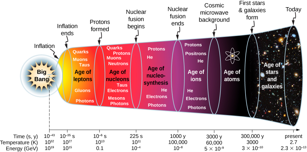
What to notice: The early universe changes state as it expands and cools. Nucleosynthesis happens early, the cosmic microwave background is released later when atoms form, and stars and galaxies appear much later. (Credit: User-provided course asset)
Track A (Core, ~30 min): Read Parts 1–7 in order, including the Hubble-law and redshift equations, Quick Checks, and final exit ticket. This gives you the expansion-history argument.
Track B (Full, ~40 min): Read everything in Track A, then spend extra time on the deep-field, CMB, and periodic-table figures. For each one, write the observation before you write the inference.
Both tracks cover the learning objectives. Track B adds more practice treating cosmology as an evidence chain instead of a set of spectacular images.
Part 1: Distance First, Then Expansion
Imagine observing a galaxy spectrum and seeing that its lines are redshifted. That tells you the light has been stretched. But by itself, it does not yet tell you the expansion history of the universe. To discover a pattern, you need distances.
This is why the distance ladder matters. Nearby methods calibrate farther-reaching methods. Parallax calibrates local stars. Cepheids extend the ladder because their pulsation periods reveal their luminosities. Supernovae extend it farther still because they can be seen across enormous distances.
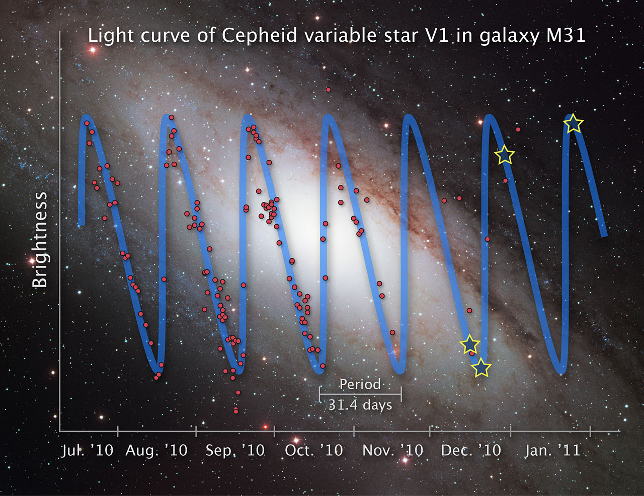
What to notice: Cepheids are useful because their brightness varies periodically. The period is the observable that calibrates their luminosity. (Credit: ESO)
A Cepheid’s brightness rises and falls in a regular pattern. The directly measured observable is time: the pulsation period. The model is the period-luminosity relation: longer-period Cepheids are more luminous. Once we know luminosity and measure flux, the inverse-square law gives distance.
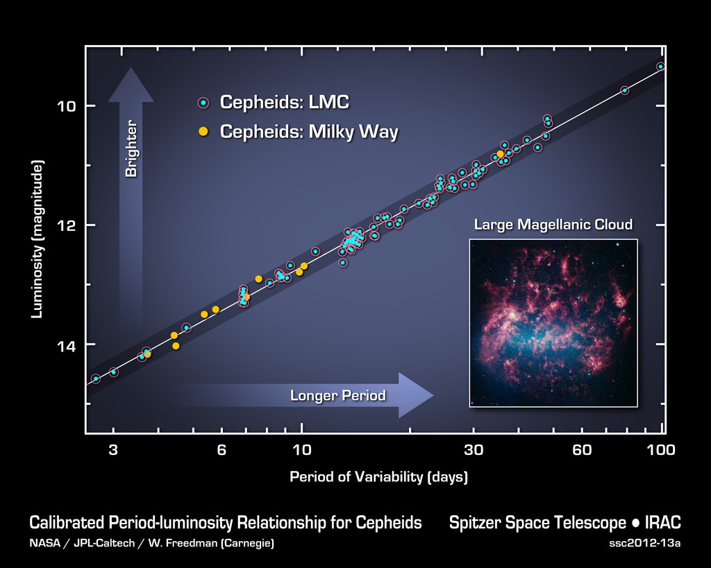
What to notice: Longer-period Cepheids are more luminous. This relation turns a time measurement into a luminosity estimate, and luminosity plus flux gives distance.
This is a beautiful example of astronomical inference. A clock-like variation becomes a luminosity. A luminosity plus a flux becomes a distance. A distance plus a redshift becomes a point on the expansion diagram.
Supernova host galaxies help extend the same logic to larger distances. The important idea is not that every standard candle is identical in every detail. The important idea is calibration. Each rung works because a lower rung teaches us how to interpret a higher rung.
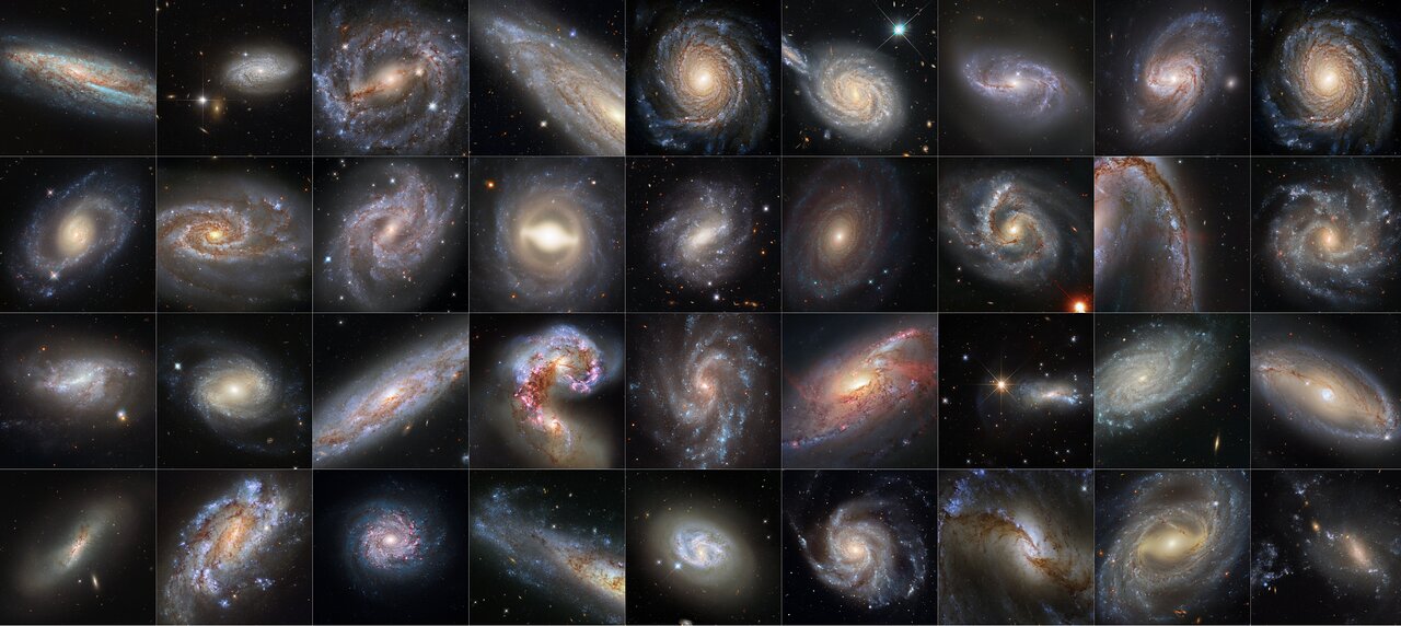
What to notice: Supernova host galaxies connect the local distance ladder to the Hubble flow. Standard candles let us compare distance and redshift far beyond the Milky Way. (Credit: NASA/ESA/Hubble/Galaxy Zoo)
Why would redshifts alone not have been enough to discover Hubble’s law?
Hubble’s law is a relation between recession speed and distance. Redshift gives the recession-speed side of the pattern, but without distances there is no way to see that more distant galaxies recede faster.
Part 2: Hubble’s Law Is an Expansion Pattern
At low redshift, the observed pattern is summarized by Hubble’s law:
\[ v = H_0 d \tag{1}\]
What it predicts
Given distance \(d\), it predicts recession speed \(v\) in the smooth Hubble flow.
What it depends on
Scales linearly: doubling distance doubles recession speed for a fixed \(H_0\).
What it’s saying
On large enough scales, more distant galaxies recede faster because the universe is expanding. The slope \(H_0\) sets the current expansion rate.
Assumptions
- Applies to large-scale cosmic expansion, not to nearby bound systems dominated by local gravity
- Uses low-redshift recession speed form; high-redshift cosmology needs the full expansion history
- \(H_0\) is measured, not predicted by this equation
See: the equation
Let’s unpack the equation. \(v\) is the recession speed inferred from redshift, usually measured in km/s. \(d\) is distance, often measured in megaparsecs for galaxies. \(H_0\) is the Hubble constant, the present-day expansion rate. The equation says that, on large enough scales, recession speed increases linearly with distance.
This is not a rule for every object near us. The Moon is not expanding away from Earth by Hubble’s law. The Solar System is bound. The Milky Way is bound. The Local Group is bound. Hubble’s law describes the large-scale expansion pattern after local gravitational motions average out.
What to notice: The Hubble constant can be inferred through multiple chains of evidence. Agreement or tension between methods is a test of the model, not just a bookkeeping detail.
The Hubble constant can be measured in more than one way. That is powerful because independent methods test the model. It is also where modern cosmology becomes alive: when different measurement chains disagree, astronomers have to decide whether the issue is unrecognized systematic error, incomplete modeling, or new physics. We do not need to solve that frontier here. We do need to understand why it matters: the expansion rate is not just a number; it is a constraint on cosmic history.
If distance is measured in megaparsecs and \(H_0\) has units of km/s/Mpc, then:
\[ H_0 d \sim \left(\frac{\mathrm{km\,s^{-1}}}{\mathrm{Mpc}}\right) \left(\mathrm{Mpc}\right) = \mathrm{km\,s^{-1}} \]
The units match a speed, as they should.
Why does Hubble’s law work better for large-scale galaxy samples than for nearby bound systems such as the Local Group?
Nearby bound systems can have motions dominated by local gravity. Hubble’s law describes the large-scale average expansion pattern after local gravitational motions are averaged over.
Part 3: Redshift as a Scale-Factor Record
In Module 1, we learned the Doppler shift: motion along the line of sight stretches or compresses wavelengths. That model still works for many nearby objects. But on cosmological scales, there is a deeper interpretation. Light from a distant galaxy travels while the universe expands. As space expands, the wavelength of that light stretches too.
\[ \begin{aligned} z &= \frac{\lambda_{\text{obs}} - \lambda_{\text{emit}}}{\lambda_{\text{emit}}}, \\ 1 + z &= \frac{\lambda_{\text{obs}}}{\lambda_{\text{emit}}} = \frac{a_0}{a_{\text{emit}}} \end{aligned} \tag{2}\]
What it predicts
Given emitted and observed wavelengths, it predicts the redshift \(z\) and how much the universe expanded while the light traveled.
What it depends on
\(z\) is the fractional wavelength increase; the redshift factor \(1+z\) equals the ratio of today’s scale factor to the scale factor when the light was emitted.
What it’s saying
Cosmological redshift is a stretch record. Light from earlier times has been stretched along with space, so redshift connects observation to cosmic history.
Assumptions
- Redshift is dominated by cosmic expansion, not local Doppler motion
- Scale factor today is often normalized to \(a_0 = 1\)
- Interpreting distance and age from \(z\) requires a cosmological model
See: the equation
This equation has three connected ways to read the same redshift. The quantity \(z\) is the fractional wavelength increase:
\[ z = \frac{\lambda_{\text{obs}} - \lambda_{\text{emit}}}{\lambda_{\text{emit}}}. \]
The quantity \(1+z\) is the total stretch factor, the ratio of observed wavelength to emitted wavelength. If a spectral line was emitted at one wavelength and observed at a longer wavelength, the redshift tells us how much the wavelength stretched. The final part connects that stretch to the scale factor \(a\), which describes the relative size of the universe at a given cosmic time.
If we set today’s scale factor to \(a_0 = 1\), then light emitted when the universe had scale factor \(a_{\text{emit}} = 1/2\) is observed with \(1+z = 2\), or \(z = 1\). The universe doubled in scale while the light was traveling.
What to notice: In an expanding universe, large-scale distances stretch with time. The galaxies are not flying through a pre-existing space in the simple everyday sense; the scale of space changes.
The Big Bang model is not a picture of galaxies flying outward from one central point into empty space. It describes the expansion and cooling of the universe itself from a hot dense early state. On large scales, every observer sees distant galaxies participating in the expansion, so there is no special center in ordinary space.
What to notice: Cosmological redshift stretches wavelengths by the expansion factor. A galaxy’s spectrum carries a timestamp from when its light was emitted. (Credit: NASA/ESA/CSA/STScI)
Cosmological redshift is therefore a time-and-scale clue. It tells us that the light we receive has crossed an evolving universe. To turn redshift into a precise distance or age, we need a cosmological model, including the effects of matter, radiation, curvature if present, and dark energy. But the core idea is already enough for this course: redshift records expansion.
If today’s scale factor is \(a_0 = 1\) and light was emitted when \(a_{\text{emit}} = 1/4\), what redshift do we observe?
If a galaxy has redshift \(z = 3\), what is the wavelength stretch factor \(1+z\)? What does that mean in scale-factor language?
The stretch factor is \(1+z = 4\). The observed wavelengths are four times longer than when emitted. In scale-factor language, the universe was one-fourth its present scale when the light was emitted, assuming today’s scale factor is normalized to 1.
Part 4: Looking Far Away Means Looking Back
Light travels at a finite speed. That simple fact turns distance into time. When we observe a nearby object, we see it as it was a short time ago. When we observe a distant galaxy, we see it as it was millions or billions of years ago.
Deep fields make this idea visible. They contain galaxies at many distances, which means they contain galaxies at many lookback times. A single image becomes a layered history of galaxy formation and evolution.
What to notice: A deep field is a time machine. Faint galaxies in the same image can be billions of years apart in lookback time. (Credit: NASA/ESA/Hubble)
This is one of the most important habits in cosmology: do not read a deep field as a flat photograph. Read it as a time archive. A small, faint, red galaxy in the background may not be a small faint version of a nearby galaxy. It may be a distant galaxy observed when the universe was much younger, with its light stretched and dimmed by cosmic expansion.
JWST pushes this logic closer to the first generations of galaxies. Very high-redshift objects test how quickly stars, gas, dust, and black holes assembled after the Big Bang.
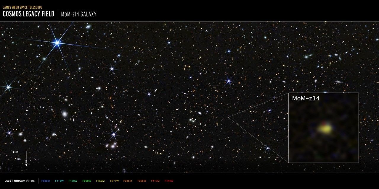
What to notice: Very high-redshift galaxies let us test how quickly structure formed after the Big Bang. The farther back we look, the closer we get to the first generations of galaxies. (Credit: NASA/ESA/CSA/STScI)
The frontier is exciting because it is a stress test. If galaxies appear earlier, brighter, or more massive than expected, then models of early galaxy formation must explain how gas cooled, formed stars, and assembled structure quickly enough. As always, the observation is not the final answer. The observation is the constraint that the model must survive.
Why should we read a deep field as a time archive rather than a flat collection of galaxies?
Because light travel time matters. More distant galaxies are seen as they were farther in the past, so a deep field mixes nearby recent galaxies with distant galaxies observed when the universe was younger.
Part 5: The Cosmic Microwave Background
If the universe was once hot and dense, then early on it should have been filled with radiation and ionized matter. At high temperatures, electrons could not remain bound to nuclei; photons scattered constantly from free electrons. The universe was opaque.
As the universe expanded, it cooled. Eventually electrons combined with nuclei to form neutral atoms. Once that happened, photons could travel freely. Those photons are still arriving today, stretched by expansion into microwave wavelengths. We call this relic radiation the cosmic microwave background, or CMB.
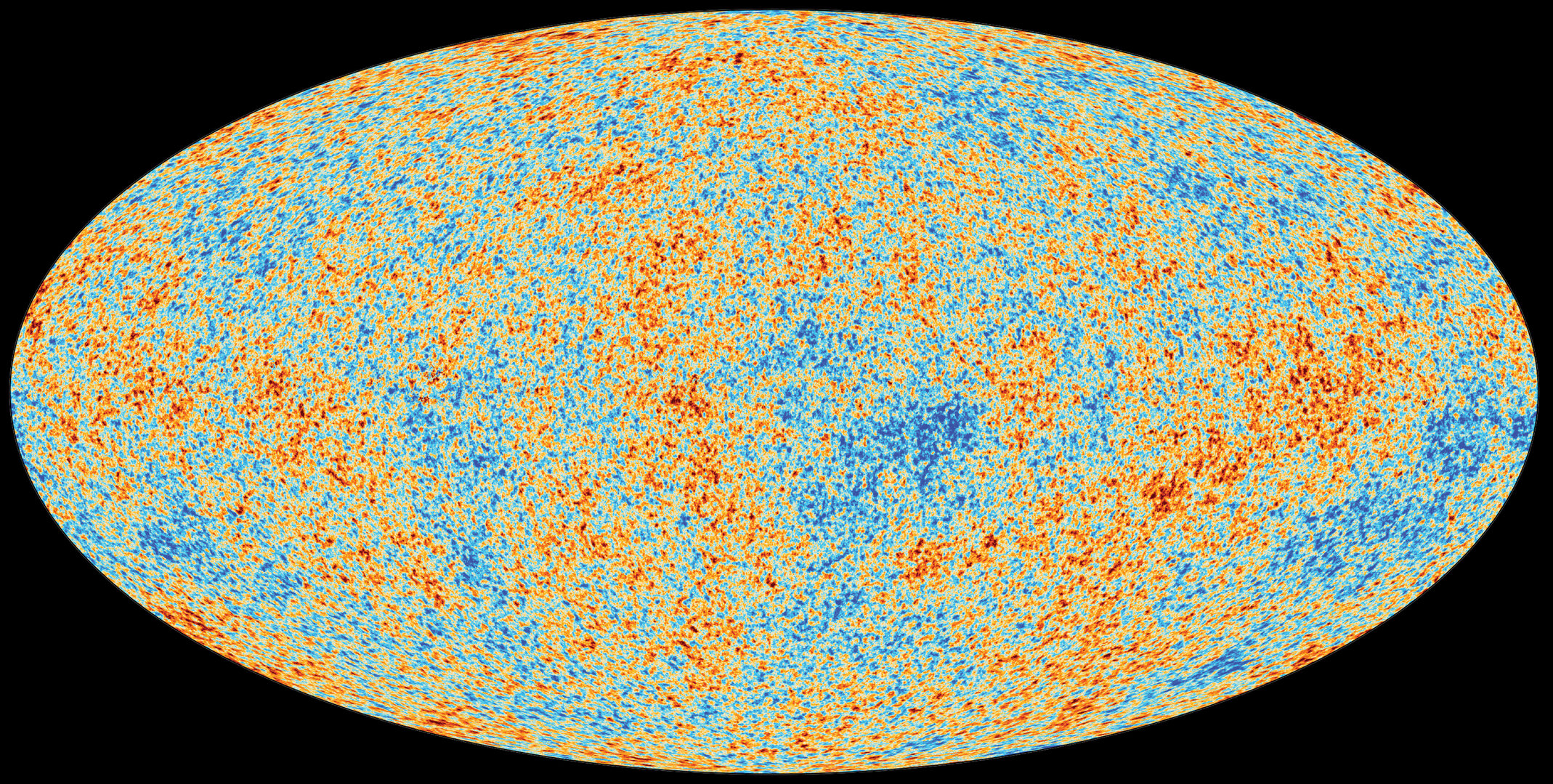
What to notice: The CMB is the most perfect blackbody ever measured (T = 2.725 K). These color variations show temperature fluctuations of only ±0.0002 K — the seeds of all cosmic structure. (Credit: ESA/Planck Collaboration)
The CMB is powerful evidence because it is not just “old light.” It has the spectrum expected from a hot dense early universe that cooled by expansion.
.jpg)
What to notice: The CMB spectrum follows a nearly perfect 2.73 K blackbody curve. This is why the CMB is evidence for a hot, dense early universe that cooled by expansion, not just a collection of old photons. (Credit: User-provided course asset)
Its tiny temperature variations are also seeds of structure: slightly denser regions that gravity could later amplify into galaxies, clusters, and the cosmic web. The cosmic web is the large-scale pattern of filaments, walls, clusters, and voids traced by galaxies today. In this reading, it matters because it connects early-universe physics to the later structure we can map with redshift surveys.
This connects directly back to the previous reading. The cosmic web did not appear from nowhere. It grew from small initial density variations under gravity. Dark matter helped structure grow; ordinary matter later cooled into galaxies and stars within that gravitational scaffolding.
Observable: microwave radiation coming from every direction, with a nearly uniform temperature plus tiny fluctuations.
Model: the universe was once hot, dense, ionized, and opaque; expansion cooled it until photons could travel freely.
Inference: the CMB is relic light from an early hot phase and contains the seeds of later structure.
What makes the CMB stronger evidence than simply saying, “the universe has old light in it”?
The CMB has the expected properties of radiation from a hot dense early universe that cooled by expansion, and its tiny temperature variations connect to the later growth of structure. It is not just old; it matches a physical model.
Part 6: The First Three Minutes
Now we arrive at the course finale: the origin of the first nuclei.
In Module 3, we studied how stars generate energy by fusing light nuclei into heavier ones. Stars make carbon, oxygen, silicon, iron, and many other elements through stellar burning and explosions. But stars did not make most of the universe’s hydrogen and helium. Those were already present before the first stars formed.
In the hot early universe, the temperature was high enough for nuclear reactions. As the universe expanded and cooled, protons and neutrons could combine into light nuclei. This era is called Big Bang nucleosynthesis, or BBN. It happened during the first few minutes, before the universe became too cool and too diffuse for those reactions to continue efficiently.
.jpg)
What to notice: In very early-universe physics, temperature and particle energy set which interactions matter. This figure is an optional big-picture reminder that cosmology connects expansion history to high-energy physics. (Credit: User-provided course asset)
This figure reaches beyond what we calculate in ASTR 201, but it shows the larger pattern: as the universe cools, different physical processes become important at different times. For this reading, the key transition is the one we can connect to matter around us: the short window when light nuclei could form.
The main BBN outcome was a universe containing mostly hydrogen nuclei, which are single protons, plus deuterium, helium-3, helium-4, and trace lithium. This is not when neutral atoms formed. BBN made nuclei; neutral atoms formed much later, when the universe cooled enough for electrons to stay bound to nuclei during recombination.
The result is a universe dominated by hydrogen, with a substantial amount of helium and tiny traces of a few other light nuclei. Heavier elements had to wait for stars and stellar remnants.
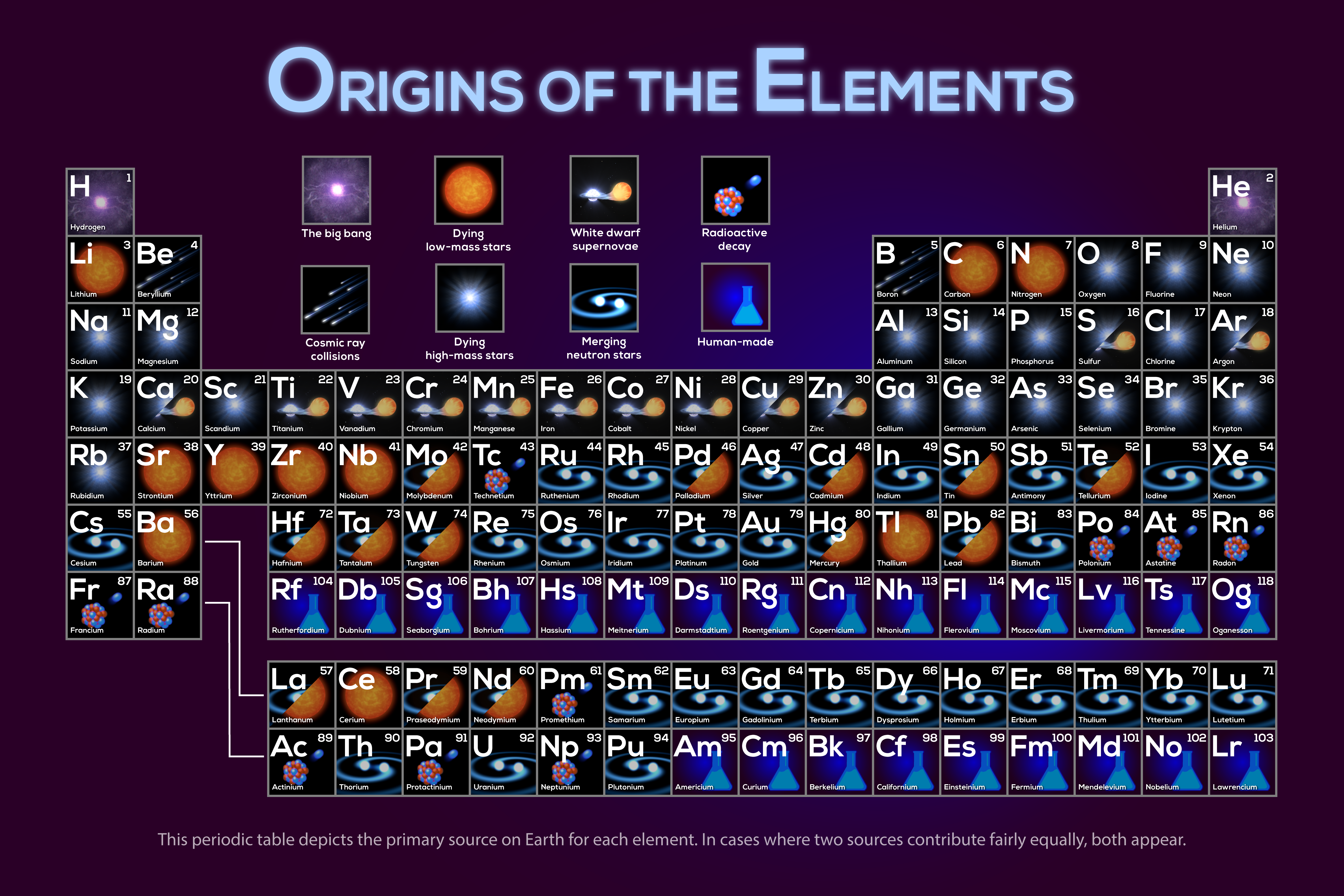
What to notice: The periodic table is a fossil record of cosmic processes. Different colors = different origins: Big Bang (H, He), dying stars (C, N, O), supernovae (Fe), neutron star mergers (Au, Pt). (Credit: NASA/Jennifer Johnson)
This figure is the punchline to the whole course. The periodic table is a fossil record of cosmic environments. Hydrogen and much of helium point back to the hot early universe. Carbon and oxygen point to stellar interiors. Iron points to advanced stellar evolution and explosions. Some of the heaviest elements point to neutron capture in extreme environments such as neutron-star mergers and certain stellar deaths.
That means you can read the matter around you as an astrophysical archive. The hydrogen in water is ancient in a different way than the oxygen in water. The hydrogen is mostly a Big Bang relic. The oxygen was forged later, inside stars. The same molecule carries multiple chapters of cosmic history.
Why is it misleading to say “stars made all the elements”?
Stars made many heavier elements, but most hydrogen and helium were produced in the early universe. Big Bang nucleosynthesis made the first light nuclei; stars and stellar remnants later made much of the rest of the periodic table.
Part 7: The Big Picture
We can now connect the full Module 4 arc.
In the first reading, galaxies were ecosystems: gas, dust, stars, and feedback cycling through time. In the second reading, gravity organized those systems and revealed hidden mass through motion, lensing, and large-scale structure. In this reading, expansion turned redshift into a history of spacetime, while the CMB and light elements pointed back to a hot dense early universe.
The course method never changed. We did not directly touch a star, a galaxy, dark matter, or the early universe. We measured signals. We built models. We inferred physical reality.
That is astronomy at its best: not a list of objects, but a discipline of disciplined imagination. The universe sends light, motion, and patterns. Physics tells us what those signals can mean. The result is a story that runs from the first nuclei to stars, galaxies, dark matter, cosmic web, and us.
Practice Problems
Use these values and ideas unless a problem states otherwise:
- At low redshift, Hubble’s law is \(v = H_0d\).
- Use \(H_0 = 70\,\mathrm{km\,s^{-1}\,Mpc^{-1}}\) for simple estimates.
- Cosmological redshift satisfies \(1+z = \lambda_{\rm obs}/\lambda_{\rm emit} = a_0/a_{\rm emit}\).
- If today’s scale factor is normalized to \(a_0 = 1\), then \(a_{\rm emit} = 1/(1+z)\).
- Light travel time means distant galaxies are seen at earlier cosmic times.
Conceptual
- ⭐ Distance before expansion.
- Why is redshift alone not enough to discover Hubble’s law?
- What role does the distance ladder play?
- Build an observe → model → infer chain for Cepheids as distance indicators.
- ⭐ Not an explosion into space. A student says, “The Big Bang happened at one point, and galaxies are flying away from that point.”
- What is misleading about that picture?
- What is expanding in the cosmological model?
- Why is there no ordinary-space center of expansion?
- ⭐⭐ CMB as evidence. Explain why the cosmic microwave background is stronger evidence than simply saying “the universe contains old light.”
Calculation
- ⭐ Using Hubble’s law. A galaxy is at distance \(d = 100\,\mathrm{Mpc}\).
- Use \(v = H_0d\) to estimate its recession speed.
- State the units of your answer.
- Explain why this estimate is more appropriate for large-scale galaxies than for the Moon or Andromeda.
- ⭐⭐ Redshift as wavelength stretch. A spectral line emitted at \(\lambda_{\rm emit} = 500\,\mathrm{nm}\) is observed at \(\lambda_{\rm obs} = 2000\,\mathrm{nm}\).
- Compute \(1+z\).
- Compute \(z\).
- If \(a_0 = 1\), what was \(a_{\rm emit}\)?
- State in words what this says about the size of the universe when the light was emitted.
- ⭐⭐ Scale factor from redshift. A galaxy has redshift \(z = 5\).
- What is the wavelength stretch factor?
- What was the scale factor when the light was emitted, assuming \(a_0 = 1\)?
- Does this calculation by itself give the exact lookback time? Why or why not?
Synthesis
- ⭐⭐ Deep fields as time archives. Choose one deep-field image from the reading. In 3–5 sentences, explain why it should be read as a history of galaxy evolution, not just a photograph of many galaxies.
- ⭐⭐ Two early-universe relics. Build two observe → model → infer chains: one for the CMB and one for light-element abundances.
- ⭐⭐⭐ The periodic table as cosmic history. Explain why hydrogen, helium, oxygen, iron, and some of the heaviest elements point to different astrophysical environments. Your answer should connect Big Bang nucleosynthesis, stellar interiors, stellar explosions, and neutron-rich extreme events.
Glossary
Big Bang nucleosynthesis: The formation of light nuclei, especially deuterium, helium-3, helium-4, and traces of lithium, during the first few minutes of the hot early universe. After BBN, most nuclei were still hydrogen nuclei, which are single protons.
Cosmic microwave background (CMB): Relic radiation from the early universe, released when the universe became transparent and later stretched into microwave wavelengths.
Cosmic web: The large-scale network of galaxy clusters, filaments, walls, and voids that grew from early density differences under gravity.
Cosmological redshift: Wavelength stretching caused by the expansion of the universe while light travels.
Distance ladder: A chain of distance-measurement methods in which nearby calibrated methods support more distant methods.
Galaxy cluster: A gravitationally bound system of many galaxies, hot X-ray-emitting gas, and dark matter.
Hubble constant (\(H_0\)): The present-day expansion rate in Hubble’s law, usually written in \(\mathrm{km\,s^{-1}\,Mpc^{-1}}\).
Hubble’s law: The large-scale relation \(v = H_0d\), connecting galaxy recession speed and distance at low redshift.
Lookback time: The time light has spent traveling from an object to us, so distant objects are seen as they were in the past.
Recombination: The era when electrons combined with nuclei to form neutral atoms, allowing photons to travel freely.
Scale factor (\(a\)): A quantity that describes the relative size of the universe at a given cosmic time.
Spacetime: The combined description of space and time. In cosmology, expanding spacetime means the scale factor changes with time, stretching large-scale distances and the wavelengths of traveling light.
Standard candle: An object whose luminosity can be inferred, allowing distance to be estimated from observed flux.
Summary
Cosmology begins with distance and redshift. The distance ladder lets us compare how far galaxies are with how much their light is stretched. Hubble’s law reveals a large-scale expansion pattern. Cosmological redshift records the changing scale factor of the universe. Deep fields turn distance into lookback time. The CMB shows that the universe was once hot, dense, and opaque. Big Bang nucleosynthesis explains why hydrogen and helium are mostly cosmic relics, while many heavier elements are products of stars and stellar remnants.
Write a three-sentence observe → model → infer chain for the first three minutes:
- What do we observe today?
- What model connects that observation to the early universe?
- What do we infer about the origin of hydrogen and helium?